|
|
||
|
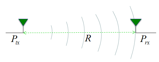
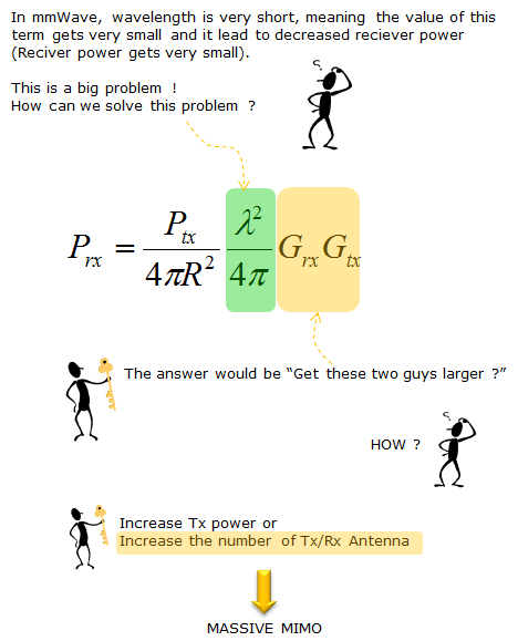
I think the main reason for Massive MIMO for 5G is 'there is no other choice'. It is highly likely that we will use very high frequency (mm Wave) signal in 5G. High frequency mean that the size of single antenna will be very small and the aperture (the area for receiving energy) will be very small. To overcome this small aperture on reciever side at high frequency, we need to use a large number of transmission antenna. This would be the main reason, but once we adopt the Massive MIMO technology, we can enjoy some other advantages coming from using a large array antenna that will be described later. Now let's look more into the meaning of 'there is no other choice'. I will describe on this aspect based on WNCG Prof. Robert Heath on Millimeter Wave MIMO Communication (I recommend you to look into the presentation on YouTube). Let's assume a situation where we have one transmission antenna and one reciever antenna placed with distance R as illustrated below.
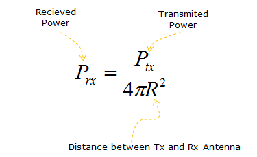
If the transmission antenna transmit signal with the power of Ptx, what would be the received signal power ? If we assume the ideal condition, the received power can be represented as follows. This would be very familiar form that you have known from high school physics, so called squared inverse rule. The received power is decreased in proportion to the square of the distance from the transmission antenna. For example, if the distance gets two times farther away, the received power gets decreased by 4 times.
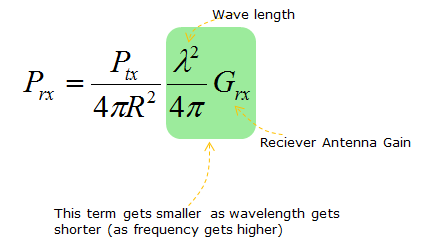
It sounds very simple. This ideal equation does not contain any parameter about frequency or the gain of the reciever antenna. It means the received signal power is not influenced by signal frequency or reciever antenna gain. But we know this is not true from our common sense in radio communication. In real life, the received signal power IS affected by the frequency (wave length) and reciever antenna gain. If we improve the mathematical model to include the frequency (wave length) and reciever antenna gain, the model can be described as shown below. According to this equation, the recieved power is in proprtion to the square of the wavelength. For example, if we assume the antenna gain does not changes, the frequency gets increased by 2 times (this mean that the wavelength gets shorten by 2 times), the recieved power gets decreased by 4 times.
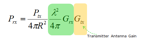
As I mentioned before, we will use much higher frequency (meaning much shorter wavelength) signal in 5G. It means the received power will be much lower than in current communication system. For example, if we use 2 Ghz frequency in current communication and we will use 20 Ghz frequency in 5G, the wavelength in 20 Ghz is 10 times shorter than the wavelength of 2 Ghz. It means the receivedpower at 20 Ghz will be 100 times lower than the received power at 2 Ghz. In reality, the situation gets even more complicated because not only the reciever antenna gain but also transmission antenna gain plays role as well. If we add the transmission antenna gain into the equation, it would become as shown below.
Now let's think of how we can overcome the drastic received power reduction at high frequency. In other words, the question is 'how we can make Prx larger ?'. Mathematically it is simple. You can get larger Prx by setting the parameters as follows. i) Increase Ptx (Transmiter Power) ii) Decrease the distance between the transmiter and reciever antenna. iii) Increase wavelength (use low frequency) iv) increase reciever antenna gain v) increase transmitter antenna gain. In real life, can we use all of these options ? The answer is 'No'. Let's look at each of these option one by one and think which one can be applicable in real life. Option i) can be doable to a certain degree, but we cannot increase the transmitter power as much as we want. Option ii) cannot be the solution since we cannot change the distance as we like. Option iii) cannot be the solution. Once we (standard organization and each Network Operator) decided to use a certain frequency, we have to follow it. We cannot change as we like. Option iv) and Option v) can be a doable solution. It may not be easy to increase the antenna gain, but at least nobody (standard organization, Network Operator) does not prevent us from trying to increase the antenna gain. Then how can we increase the antenna gain ? We may increase the antenna gain by design (e.g, shape, material etc), but the amount of gain improvement by design cannot be as large as to compensate the huge amount of the power reduction cause by the increased frequency. Almost the only way in this case would be to increase the number of antenna and it is the major motivation of using Massive MIMO as illustrated below.
In addition to increasing the received power, Massive MIMO provides several other advantages as well. According to "Massive MIMO for Next Generation Wireless Systems" ([5]), the potential (advantage) of Massive MIMO is described as follows;
I found another very well summarized list of motivation and challeges about Massive MIMO from 3GPP R1-136362 ([6]).
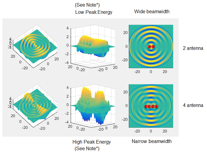
Spatial Focus with More AntennaThere is one thing that is automatically aquired by Massive MIMO. It is the fact that most of energy transmitted from the antenna array focus on very narrow area. It means the beamwidth get narrower as you use more antenna. Following plot would give you an example for the effect of beamwidht narrowing with the increased number of antenna. This effect would cause both advantage and disadvatange at the sametime. Advatantage would be that there will be less interference between beams for different users since each of the beam would be focused in very small area and the disadvantage would be that you have to implement very sophisticated algorithm to find exact location of the user and directing the beam to the user with high accuracy. (NOTE : Click on the picture for slideshow / animated version in my visual note : two difference examples are there. One for beam forming and the other one for beam steering)
Note *: In this example, I assume that each of the antenna transmit the exact same power regardless of whether it is in 2 antenna array or in 4 antenna array. So you see higher peak power in 4 antenna array. But in reality, they would decrease the transmit power for each antenna as they increase the number of antenna. The point is that you should not increase the total transmitted power from the whole array even though you increase the number of antenna. Following is the matlab source code for this example. Don't take this seriously.. this is just a toy program to give you the big picture of how antenna array works.. it would not be accurate model. Just play with it and have some fun. Save the following code in a m file named waveCosPh.m function z = waveCosPh(x,y,Ph,r) d = sqrt(x.^2 + y.^2);
dim = size(d); dr = dim(1); dc = dim(2);
for i = 1 : dr for j = 1 : dc if d(i,j) > r d(i,j) = pi/2; end; end; end; z = cos(d-Ph); end Run following code in another m file (any name is OK) that is located in the same folder as waveCosPh.m clear all;
xstep = -10*pi:pi/10:10*pi; ystep = -10*pi:pi/10:10*pi;; [X,Y] = meshgrid(xstep,ystep);
[X1,Y1] = meshgrid(xstep-pi/2,ystep); Z1 = waveCosPh(X1,Y1,0,10*pi);
[X2,Y2] = meshgrid(xstep+pi/2,ystep); Z2 = waveCosPh(X2,Y2,0,10*pi);
[X3,Y3] = meshgrid(xstep-pi/2-pi,ystep); Z3 = waveCosPh(X3,Y3,0,10*pi);
[X4,Y4] = meshgrid(xstep+pi/2+pi,ystep); Z4 = waveCosPh(X4,Y4,0,10*pi);
Z = Z1 + Z2;
subplot(2,3,1); mesh(X,Y,Z);xlim([-10*pi 10*pi]);ylim([-10*pi 10*pi]);zlim([-4,4]); view([-40 70]);
subplot(2,3,2); mesh(X,Y,Z);xlim([-10*pi 10*pi]);ylim([-10*pi 10*pi]);zlim([-4,4]); view([-40 10]);
subplot(2,3,3); mesh(X,Y,Z); xlim([-10*pi 10*pi]);ylim([-10*pi 10*pi]);zlim([-4,4]); view([0 90]);
Z = Z1 + Z2 + Z3 + Z4;
subplot(2,3,4); mesh(X,Y,Z);xlim([-10*pi 10*pi]);ylim([-10*pi 10*pi]);zlim([-4,4]); view([-40 70]);
subplot(2,3,5); mesh(X,Y,Z);xlim([-10*pi 10*pi]);ylim([-10*pi 10*pi]);zlim([-4,4]); view([-40 10]);
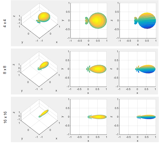
subplot(2,3,6); mesh(X,Y,Z); xlim([-10*pi 10*pi]);ylim([-10*pi 10*pi]);zlim([-4,4]); view([0 90]); Following is another toy program that shows you beam pattern out of 2 dimensional antenna array (this is linear scale, not dB scale). You would notice how narrower the beam width become as the number of antenna in the array get larger. (Note : I put more examples of various beams with varying number of antenna configuration at my visual note. See here)
Followings are the matlab code that I used to draw the pattern shown above. You may play with the code by changing M, N value. N = 16; M = 16;
phi = linspace(-pi,pi,10*N); theta = linspace(-pi,pi,10*N); [phi,theta] = meshgrid(phi,theta);
Beam = sinc(1/pi*N*phi/2)./sinc(1/pi*phi/2).*sinc(1/pi*M*theta/2)./sinc(1/pi*theta/2); Beam = abs(Beam)/max(max(abs(Beam)));
subplot(1,3,1); [x,y,z] = sph2cart(phi,theta,Beam); surface(x,y,z,'EdgeColor','none');axis([-1 1 -1 1 -1 1]); xlabel('x');ylabel('y');zlabel('z'); grid(); view(-45,70);
subplot(1,3,2); [x,y,z] = sph2cart(phi,theta,Beam); surface(x,y,z,'EdgeColor','none');axis([-1 1 -1 1 -1 1]); xlabel('x');ylabel('y');zlabel('z'); grid(); view(0,90);
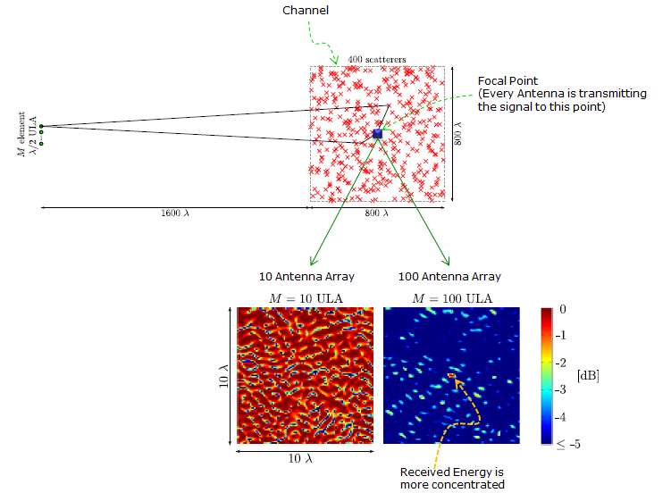
subplot(1,3,3); [x,y,z] = sph2cart(phi,theta,Beam); surface(x,y,z,'EdgeColor','none');axis([-1 1 -1 1 -1 1]); xlabel('x');ylabel('y');zlabel('z'); grid(); view(0,0); You can get more theoretical explanation about this property from various papers and following is one example based on Scaling up MIMO : Opportunities and Challenges with Very Large Arrays Following is to illustrate how large antenna arrays can focus the electromagnetic field to a certain geographic point. This specific case shows the resulting normalized field strength. (This example huses TRBF(Time-Reversal BeamForming) with MF precodings.
This result shows i) the field strength can be focused to a point rather than in a certain direction ii) more antenna improve the ability to focus engergy to a certain point With enough many antennas and favorable propagaton i) TRBF focus power and yield a high spectral efficientcy through spatial multiplexing to many terminals ii) TRBF also reduce (or completely elminate in ideal case) inter-symbol interference, meaning that we could dispense with OFDM and its redundant cyclic prefix.
Process being done by each base station antenna i) convolve the data sequence intended for the k-th terminal with the conjugated, time-reversed version of his estimate for the channel impulse response to the k-th terminal ii) sum the K convolutions iii) feed that sum into the antenna
Reference[1] GFDM Interference Cancellation for Flexible Cognitive Radio PHY Design R. Datta, N. Michailow, M. Lentmaier and G. Fettweis Vodafone Chair Mobile Communications Systems, Dresden University of Technology, 01069 Dresden, Germany Email:[rohit.datta, nicola.michailow, michael.lentmaier, fettweis]@ifn.et.tu-dresden.de [2] 5G NOW. D3.1 5G Waveform Candidate Selection
[3] Massive MIMO and Small Cells : Improving Energy Efficiency by Optimal Soft-Cell Coordination Emil Bjornson, Marios Kountouris and Merouane Debbah Alcatel-Lucent Chair on Flexible Radio, SUPELEC, Gif-sur-Yvette, France Department of Telecommunications, SUPELEC, Gif-sur-Yvette, France ACCESS Linnaeus Center, Signal Processing Lab, KTH Royal Institue of Technology, Stockholm, Sweden
[5] Massive MIMO for Next Generation Wireless Systems Erik G. Larson, ISY, Linkoping University, Sweden Ove Edfors, Lund University, Sweden Fredrik Tufvesson, Lund University, Sweden Thomas L. Marzetta, Bell Labs, Alcatel-Lucent, USA
[6] Scaling up MIMO : Opportunities and Challenges with Very Large Arrays Fredrik Rusek, Dept. of Electrical and Information Technology, Lund University, Lund, Sweden Daniel Persson, Dept. of Electrical Engineering (ISY), Linkoping University, Sweden Buon Kiong Lau, Dept. of Electrical and Information Technology, Lund University, Lund, Sweden Erik G. Larsson, Dept. of Electrical Engineering (ISY), Linkoping University, Sweden Thomas L. Marzetta, Bell Laboratories, Alcatel-Lucent, Murray Hill, NJ Ove Edfors, Dept. of Electrical and Information Technology, Lund University, Lund, Sweden Fredrik Tufvesson, Dept. of Electrical and Information Technology, Lund University, Lund, Sweden
[7] 3GPP TSG-RAN WG1 #85 R1-165362 : Multi-Antenna Architectures and Implementation issues in NR
[8] Massive Mimo Blog by EMIL BJRNSON
|
||