5G - Waveform Candidate - FBMC - 5G

5G - PHY Candidate Home : www.sharetechnote.com

FBMC(Filter-bank based multi-carrier)

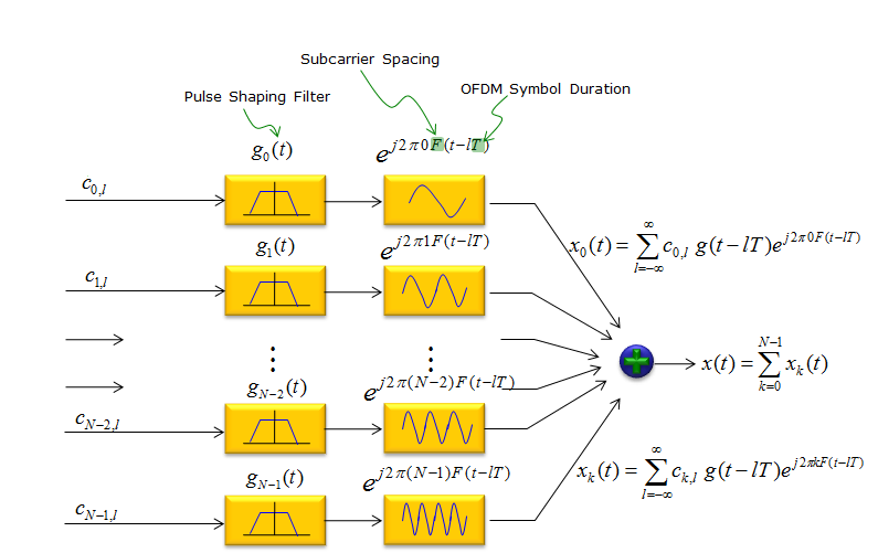
In this scheme, a filter is applied per sub carrier and can be modeled as shown below.

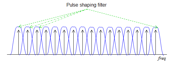
The process illustrated above can be represented in more intuitive way as shown below. As you see, each of sub channel goes through a bandpass filter.

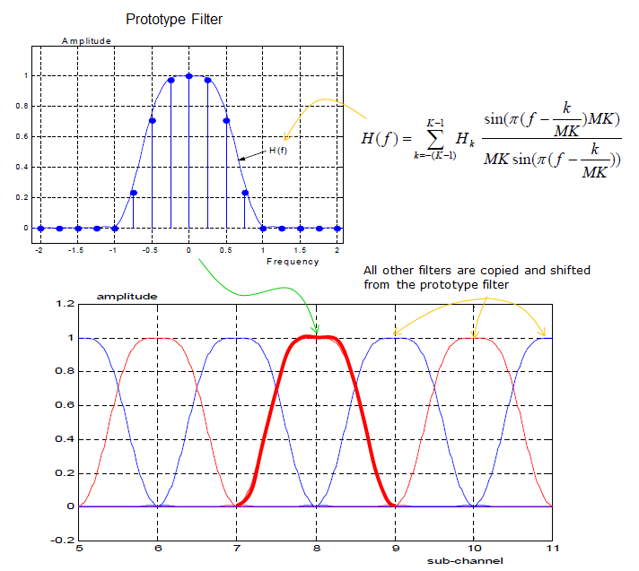
The critical steps for FBMC is to implement filters for each sub channels and align the multiple filters into a filter bank. The way to build the filter bank is .. we design a basic form (template) of a filter called prototype filter. Once we finish the design of the prototype filter, the next step is simple. Just make a copy of the prototype filter and shift it to neighbouring sub channels step by step. (Following illustration is based on Ref [4])

Example 01 >

Following is an example of generating FBMC signal. The generation part came from Michel TERRE's Matlab code (Refer to Ref [5] for original code and Copyright Info). I added plotting parts and I will describe on each of the steps.

clear all;

close all;

clc;

N=16;

% Prototype Filter (cf M. Bellanger, Phydyas project)

H1=0.971960;

H2=sqrt(2)/2;

H3=0.235147;

factech=1+2*(H1+H2+H3);

hef(1:4*N)=0;

for i=1:4*N-1

hef(1+i)=1-2*H1*cos(pi*i/(2*N))+2*H2*cos(pi*i/N)-2*H3*cos(pi*i*3/(2*N));

end

hef=hef/factech;

% Prototype filter impulse response

h=hef;

% Initialization for transmission

Frame=1;

y=zeros(1,4*N+(Frame-1)*N/2);

s=zeros(N,Frame);

for ntrame=1:Frame

% OQAM Modulator

if rem(ntrame,2)==1

s(1:2:N,ntrame)=sign(randn(N/2,1));

s(2:2:N,ntrame)=j*sign(randn(N/2,1));

else

s(1:2:N,ntrame)=j*sign(randn(N/2,1));

s(2:2:N,ntrame)=sign(randn(N/2,1));

end

x=ifft(s(:,ntrame));

% Duplication of the signal

x4=[x.' x.' x.' x.'];

% We apply the filter on the duplicated signal

signal=x4.*h;

%signal=x4;

% Transmitted signal

y(1+(ntrame-1)*N/2:(ntrame-1)*N/2+4*N)=y(1+(ntrame-1)*N/2:(ntrame-1)*N/2+4*N)+signal;

end

yfft = [zeros(1,length(y)/2) fft(y) zeros(1,length(y)/2)]

yTx = ifft(yfft);

yTxFreq = fft(yTx,8192);

yTxFreqAbs = abs(yTxFreq);

yTxFreqAbs = yTxFreqAbs/max(yTxFreqAbs);

yTxFreqAbsPwr = 20*log(yTxFreqAbs);

subplot(6,4,1); plot(h);xlim([0 length(h)]);set(gca,'yticklabel',[]);

subplot(6,4,2); plot(s);xlim([-1.2 1.2]);ylim([-1.2 1.2]);set(gca,'yticklabel',[]);

subplot(6,4,3); stem(real(s));xlim([1 length(s)]);ylim([-1.2 1.2]);set(gca,'yticklabel',[]);

subplot(6,4,4); stem(imag(s));xlim([1 length(s)]);ylim([-1.2 1.2]);set(gca,'yticklabel',[]);

subplot(6,4,5); plot(real(x));xlim([1 length(x)]);set(gca,'yticklabel',[]);

subplot(6,4,6); plot(imag(x));xlim([1 length(x)]);set(gca,'yticklabel',[]);

subplot(6,4,7); plot(real(x4));xlim([0 length(x4)]);ylim([-0.5 0.5]);set(gca,'yticklabel',[]);

subplot(6,4,8); plot(imag(x4));xlim([0 length(x4)]);ylim([-0.5 0.5]);set(gca,'yticklabel',[]);

subplot(6,4,9); plot(real(signal));xlim([0 length(signal)]);ylim([-0.5 0.5]);set(gca,'yticklabel',[]);

subplot(6,4,10); plot(imag(signal));xlim([0 length(signal)]);ylim([-0.5 0.5]);set(gca,'yticklabel',[]);

subplot(6,4,11); plot(real(y));xlim([0 length(y)]);ylim([-0.5 0.5]);set(gca,'yticklabel',[]);

subplot(6,4,12); plot(imag(y));xlim([0 length(y)]);ylim([-0.5 0.5]);set(gca,'yticklabel',[]);

subplot(6,4,13); plot(real(yfft));xlim([0 length(yfft)]);set(gca,'yticklabel',[]);%ylim([-0.5 0.5]);

subplot(6,4,14); plot(imag(yfft));xlim([0 length(yfft)]);set(gca,'yticklabel',[]);%ylim([-0.5 0.5]);

subplot(6,4,15); plot(abs(yfft)/max(abs(yfft)));xlim([0 length(yfft)]);set(gca,'yticklabel',[]);%ylim([0 1]);

subplot(6,4,16); plot(20*log(abs(yfft)/max(abs(yfft))));xlim([0 length(yfft)]);set(gca,'yticklabel',[]);%ylim([-10 0]);

subplot(6,4,17); plot(real(yTx));xlim([0 length(yTx)]);set(gca,'yticklabel',[]);%ylim([-0.5 0.5]);

subplot(6,4,18); plot(imag(yTx));xlim([0 length(yTx)]);set(gca,'yticklabel',[]);%ylim([-0.5 0.5]);

subplot(6,4,19); plot(abs(yTx)/max(abs(yTx)));xlim([0 length(yTx)]);ylim([0 1]);set(gca,'yticklabel',[]);

subplot(6,4,20); plot(20*log(abs(yTx)/max(abs(yTx))));xlim([0 length(yTx)]);ylim([-100 0]);set(gca,'yticklabel',[]);

subplot(6,4,21); plot(real(yTxFreq));xlim([0 length(yTxFreq)]);set(gca,'yticklabel',[]);%ylim([-0.5 0.5]);

subplot(6,4,22); plot(imag(yTxFreq));xlim([0 length(yTxFreq)]);set(gca,'yticklabel',[]);%ylim([-0.5 0.5]);

subplot(6,4,23); plot(yTxFreqAbs);xlim([0 length(yTxFreqAbs)]);ylim([0 1]);set(gca,'yticklabel',[]);

subplot(6,4,24);plot(yTxFreqAbsPwr); xlim([0 length(yTxFreqAbsPwr)]);ylim([-100 0]);set(gca,'yticklabel',[]);

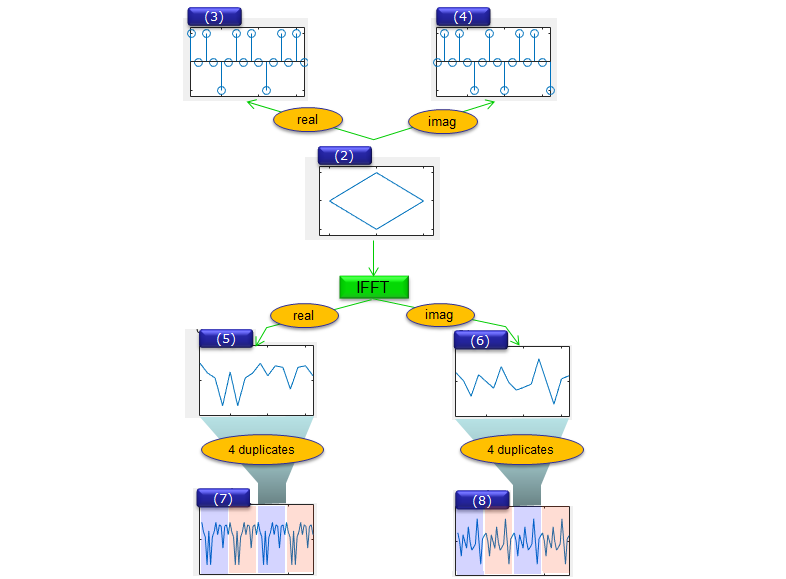
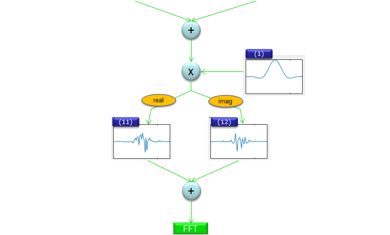
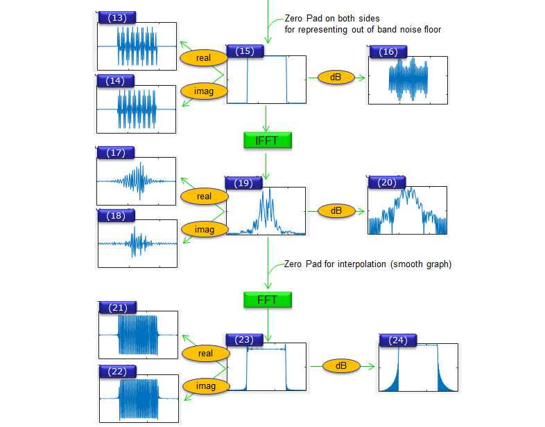
Following is the output of this code. The 'X' of subplot(6,4,X) corresponds to the number in following graphs. First, try to understand on your own the meaning of each of these plots based on the source code and then follow through my description.

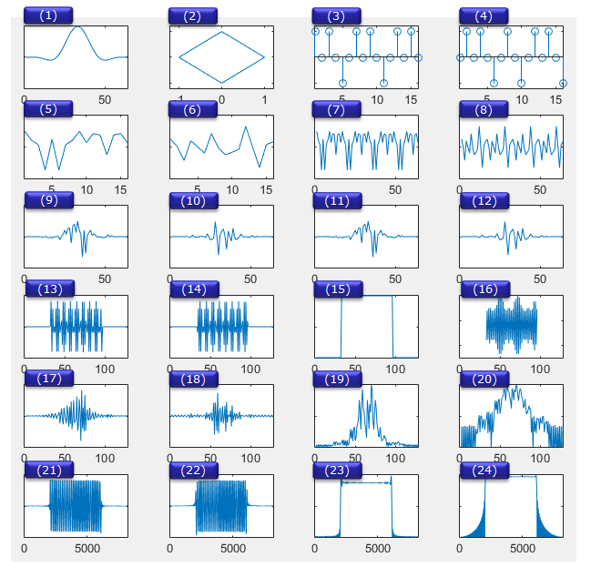
Following shows how each of the plots are produced along the each steps of FBMC waveform generation. I hope this would be clearer than any verbal (written description).

Just putting the important milestone points, (2) is the bit stream mapped to a sequence of complex data and represnted in constallation. (1) is Pulse Shaping Filter. (19) is the time domain physical signal being transmitted through the antenna after upconversion. (21) is the time domain physical signal being transmitted through the antenna after upconversion.

Reference

[1] GFDM Interference Cancellation for Flexible Cognitive Radio PHY Design

R. Datta, N. Michailow, M. Lentmaier and G. Fettweis

Vodafone Chair Mobile Communications Systems,

Dresden University of Technology,

01069 Dresden, Germany

Email:[rohit.datta, nicola.michailow, michael.lentmaier, fettweis]@ifn.et.tu-dresden.de

[2] 5G NOW. D3.1 5G Waveform Candidate Selection

[3] Waveform Contenders for 5G - suitability for short packet and low latency transmissions.

Frank Schaich, Thorsten Wild, Yegian Chen

Alcatel-Lucent AG

Bell Labs

Stuttgart, Germany

[4] FBMC Physical Layer : a Primer

PHYDYAS

[5] Matlab Centeral : FBMC Modulation / Demodulation (with BSD Copyright)

Copyright (c) 2014, Michel TERRE
All rights reserved.