MMSE is a model that minimize the MSE (Mean Square Error) of the received data. With this single statement, a lot of questions would start popping up in your mind.
What is Mean Square Error ? What is the physical meaning of 'minimized MSE' ? etc.
The Minimum Mean Squared Error (MMSE) equalizer is a linear equalization technique used in digital communication systems to mitigate the effects of inter-symbol interference (ISI) and noise. The MMSE equalizer is designed to minimize the mean squared error between the transmitted signal and the equalized received signal.
In the context of a Multiple-Input Multiple-Output (MIMO) system, let's consider the following linear equation representing the received signal Y, transmitted signal X, channel matrix H, and noise vector N:
Y = H * X + N
The goal of the MMSE equalizer is to find an equalization matrix W_mmse that minimizes the mean squared error between the transmitted signal X and the equalized received signal W_mmse * Y:
W_mmse = argmin ||X - W_mmse * Y||2
In contrast to the Zero Forcing (ZF) equalizer, which only focuses on inverting the channel matrix H to eliminate ISI, the MMSE equalizer balances the elimination of ISI with controlling the noise amplification. This is achieved by minimizing the mean squared error between the transmitted and equalized signals, which considers both the ISI and the noise. This makes the MMSE equalizer more robust to noise compared to the ZF equalizer.
The MMSE equalizer matrix can be computed as follows:
W_mmse = H' * inv(H * H' + N0 * I)
,where H' is the Hermitian (conjugate) transpose of H,
N0 is the noise power (This is not a direct noise power, check the NOTE below)
I is the identity matrix.
Note that the noise power N0 is an important factor in the MMSE equalization process, as it helps to balance the trade-off between ISI suppression and noise amplification.
The MMSE equalizer generally outperforms the ZF equalizer in noisy environments, as it aims to minimize the overall mean squared error, taking both ISI and noise into account. However, the MMSE equalizer is more computationally complex due to the need to estimate the noise power and compute the matrix inversion.
Finally we can get the estimated Tx signal X from W_mmse and Y(recieved signal) as follows :
Xest = W_mmse * Y
NOTE : How can I figure out which value to use for N0 ? The performance of the MMSE equalizer depends on an accurate estimate of N0. If the noise power is overestimated or underestimated, the equalizer may not achieve the best trade-off between ISI suppression and noise amplification. In practice, iterative or adaptive algorithms can be used to refine the noise power estimate and improve the performance of the MMSE equalizer.
There are a few different approaches listed below.
- Measurements: Measure the noise power directly in the system. This can be done by collecting samples of the received signal when the transmitter is off or by measuring the noise floor of the receiver. The variance of the noise samples can be used as an estimate for N0.
- Channel estimation: If your system employs a known training sequence or pilot symbols, you can use these known signals to estimate the channel and noise characteristics. By comparing the received training sequence with the transmitted one and computing the error, you can estimate the noise power N0.
- SNR calculations: If you know the signal-to-noise ratio (SNR) at the receiver, you can compute the noise power N0 based on the received signal power. For example, if the received signal power is P_r and the SNR is given in dB, you can calculate N0 as follows:
SNR_linear = 10^(SNR_dB / 10);
N0 = P_r / SNR_linear;
Looking in a little bit detail
Let's start with a channel model that we got very familiar by now. (I hope you are now familiar with the following expression as well.)
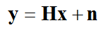
MMSE as an Equalizer is a kind of post processing algorithm that helps us to figure out the received data that is as close to the original data (transmitted data) as possible. In short, the most important steps in MMSE is to find a matrix G in the following illustration. If we assume that there is no noise, this [G] matrix can be simply an inverse of channel matrix (H-1). But when there is noise, we would need to use some model that can reflect the noise. MMSE is one of these algorithms.
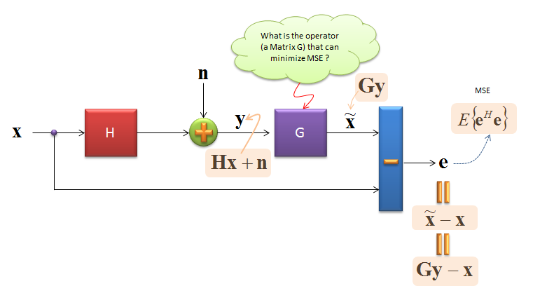
Now we set a goal meaning that we have a kind of goal function to solve. Then, we need to figure out how to solve the goal function. There are several different approach to reach the solution. The approach I would take is to solve following equation.
When I first learned about this equation, my first question was what is the meaning of this equation. If you take a little closer look at it, you would realize that these equation indicate a specific condition where there is no correlation between the received data vector and error vector.
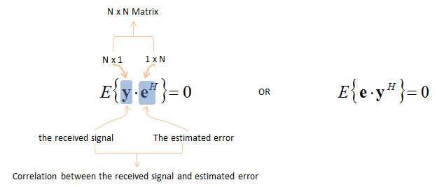
My next question was 'how this specific condition becomes the condition to minimize the MSE of the error ?', in short 'how this can be the condition for MMSE ?'.
Following is the comment from a FPGA engineer who teaches me in various topics in physical layer. It may not sound so clear at the first reading, but give some more thought on it and it would start making sense.
In MMSE, the matrix G shall be such a matrix that minimizes the MSE by utilizing the statistical characteristics of the received signal. If there remains some correlation between “y” and “e”, the correlation should be able to be utilized for decreasing the norm of “e”. So, at the optimum point, there should be no correlation between “y” and “e”. ( If not, we should be able to decrease the norm of “e” even more by utilizing the correlation.)
This is the reason why we can derive the MMSE-optimal matrix G by using the criteria that claims that the correlation between the received signal “y” and the error “e” is zero.
Once you get the object equation to solve and understand the physical (or statistical) meaning of it, the remaining step is just high school math. One advise I would give you is 'Don't think too much of physical meaning of the solution process until you reach the final solution'. Most of the intermediate steps are purely mathematical manipulation and in most case there is no specific physical meaning. Of course, there are some cases where we need to think of physical meaning, for example when removing some terms in the solution process. But in most case, this solution process is just mathematical manipulation.
First, you can expand the object equation given to us as shown in the following process. Don't get intimidated, just pull out a sheet of paper and a pen, write down each step by hands. You would learn it is a really high school math.
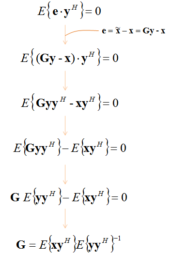
Now we have the matrix [G] expressed in two blocks of E{ }. Let's expand each of these blocks further.
Then you may ask why have have to do more expansion ? why we cannot use this result as a solution ?
To use this as a solution, you need to know all the values in the equation.
Let's look into each terms in this (the last line above) and check if we know all the values.
Can we know of [y] vector ? Yes, because it is the value that has been first physically detected/measured by the reciever.
How about [x] vector ? It is transmitted data. If this transmitted data is a reference signal, we can say we know the value, but if it is user data, we don't know of the value.
Now let's expand each of E{ } blocks one by one. Let me try with the second E{ } block first. (there is no specific reason why I expand the second block first.. I just did it :). In this process, you see some of the terms (marked in color) were removed and were replaced by other simpler form. This is based on the physical properties of the terms. There is no purely mathematical reason on how you can remove or replace those terms.
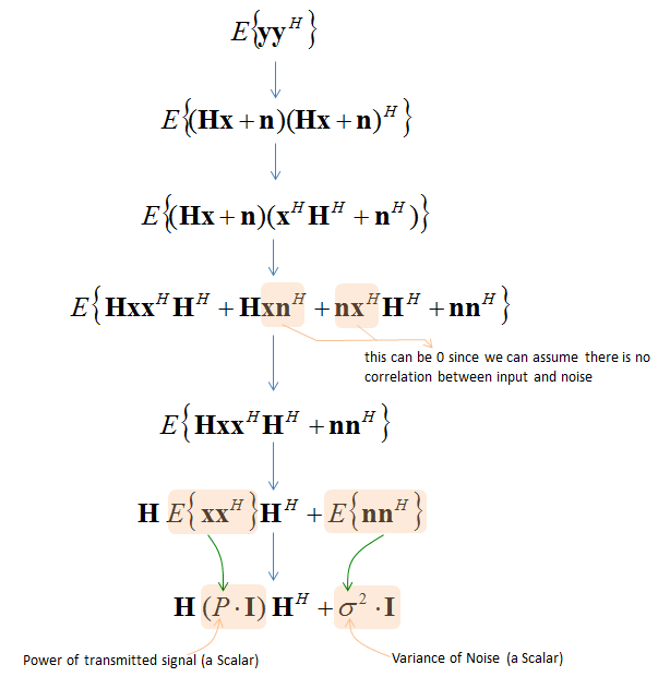
Now we have the expression that is made up of values that is known to us. [H] is the channel matrix. We assume that we already figured out this matrix during the channel estimation process. We know P since we determines transmission power. How about 'Variance of Noise' ? We would not be able to know exact noise value added to each and every received data, but we can figure out the long term statistical property of the noise. 'Variance of Noise' is a kind of long terms statistical properties of the noise.
Next, let's expand the first E{ } block. It can be expanded as shown below. In this process as well, you see some of the terms (marked in color) were removed and were replaced by other simpler form. This is based on the physical properties of the terms
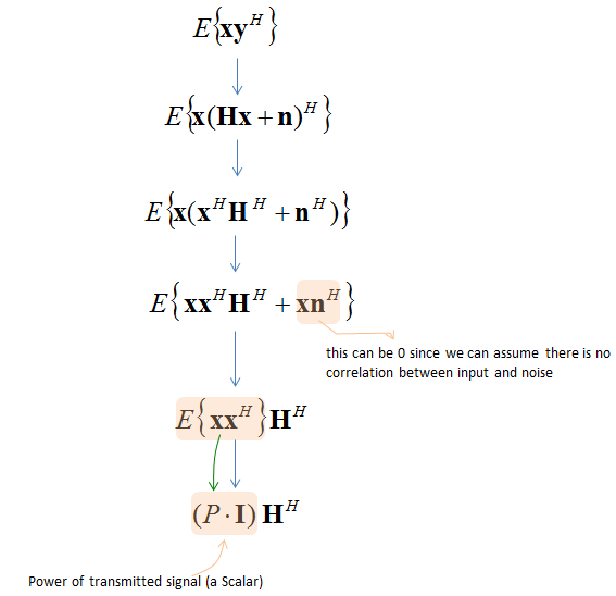
Now that we have the expanded form of both E{ } blocks, let rewrite [G] matrix using the expanded expression and it become as follows.
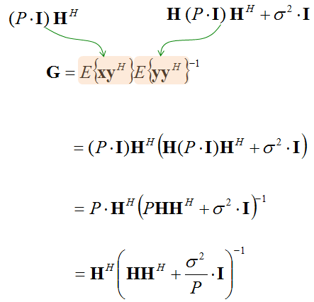
Now you see the whole [G] matrix itself is represented with all the known values. In real DSP or FPGA to solve this expression, you may need further manipulation (e.g, Matrix Decomposition), but just for understanding the concept of MMSE this would be enough.
One big question at this point even if you folowed through this long/boring math process would be 'In order to derive G, we reached the conclusion that we need to know the channel matrix H. How can we know of it ?'. This is where you need to study another complicated and boring topic called 'Channel Estimation'.
NOTE : The interpretation of H in the equation above varies a little depending on the implemenation of the system. If we assume a system without doing any amplification nor precoding, the H represents only the properties of over the air channel as illustrated here. But if we assume a more realistic implementation which perform some precoding and amplification, the H indicate a matrix that include the property of precoding and amplification. Mathematically the H in this case can be expressed as 'Amp * H * P', where Amp is amplification, H is channel matrix over the air and P is precoding matrix.
If you are interested in getting some example of MMSE implementation, see this page. I posted some of Matlab examples of MMSE equalization.
MMSE Application - LTE
The equations above describe MMSE in general terms. LTE fixes the notation and the receiver structure, so the same idea appears here in a concrete form. Every version below uses the same equalizer. They differ only in the covariance matrix R that feeds it, and that one choice decides how well the receiver can reject interference from the neighbouring cells.
This is based on TR 36.829 V11.1.0 (2012-12)
Reciever Chain Process
The starting point is the received vector at one resource element. The equation below splits it into three contributions, and the middle one is what separates the LTE case from the textbook case.
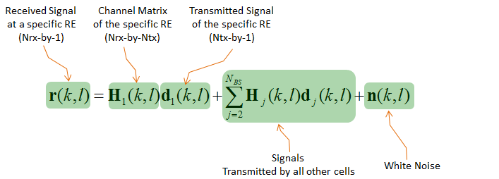
- r(k,l) is the received signal at a specific RE, with dimension Nrx by 1. The index pair (k,l) fixes one subcarrier and one symbol.
- H1(k,l) d1(k,l) is the wanted term. H1 is the channel matrix of the specific RE, Nrx by Ntx, and d1 is the transmitted signal of that RE, Ntx by 1.
- The sum from j = 2 to NBS holds the signals transmitted by all other cells. Each one reaches the antenna through its own channel matrix Hj.
- n(k,l) is the white noise, and it is the only disturbance the baseline receiver models explicitly.
The receiver recovers the data with one matrix multiplication. Everything the receiver can do about interference is therefore decided by the contents of that single matrix.
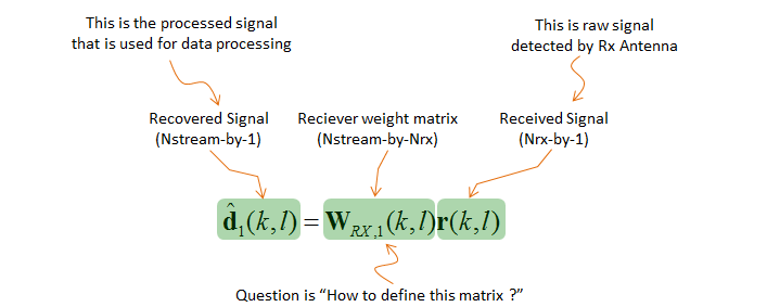
- The left side is the recovered signal, written as d1 with a hat, with dimension Nstream by 1. The note above it calls this the processed signal that is used for data processing.
- WRX,1(k,l) is the reciever weight matrix, Nstream by Nrx.
- r(k,l) is the raw signal detected by the Rx antenna, unchanged from the equation above.
The question printed under the drawing is what the rest of this section answers. How should that weight matrix be defined ?
The MMSE answer splits the weight matrix into two parts. One part is the estimated channel, written as H1 hat, and the other is the inverse of a covariance matrix R.

The note in the drawing states the point plainly. The efficiency of W is determined by how R is defined, so the three versions that follow differ in that one expression and in nothing else.
MMSE : Baseline
The baseline definition counts two things. The first is the wanted signal, scaled by its transmit power P1. The second is white noise with variance sigma squared, spread evenly across the receive antennas.

Nothing in that expression describes the other cells. A receiver built this way treats their contribution as if it were white noise, so it cannot steer a null towards any of them.
MMSE : IRC
IRC stands for Interference Rejection Combining, and it changes exactly one term. The white noise term gives way to a measured covariance, taken from the part of the received signal that the wanted channel does not account for.
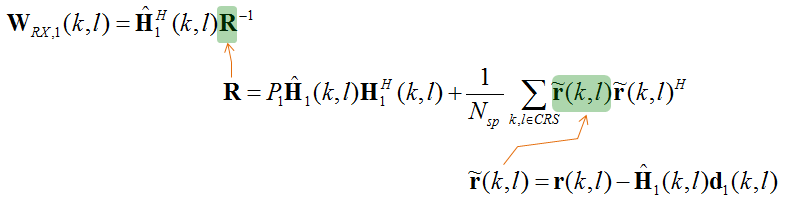
The residual, written as r with a tilde, is the received vector minus the reconstructed wanted signal. What remains holds the other cells and the noise together. Averaging that residual against its own Hermitian transpose over Nsp resource elements therefore measures the interference the receiver actually faces. In the version above the sum runs over the CRS positions.
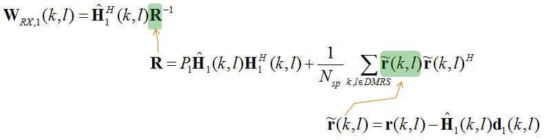
The version above is the same construction taken over DMRS positions rather than CRS. DMRS carries the same precoding as the data beside it, so a residual measured there reflects the interference that the data sees. CRS is common to the whole cell and carries no precoding, so the two estimates can differ whenever the transmitter uses beamforming.
The last version drops the reconstruction step. It builds R straight from the received samples, without subtracting the wanted term first, and it averages over the PDSCH and DMRS resource elements together.

The four definitions line up as follows.
- Baseline. R is P1 H1 hat H1H plus sigma squared times the identity matrix. The interference is never measured, only assumed to be white.
- IRC on CRS. The noise term becomes an average of the residual covariance over the CRS resource elements.
- IRC on DMRS. The same average, taken over the DMRS resource elements.
- Direct estimate. R is the average of r rH over the PDSCH and DMRS resource elements, with no subtraction at all.
The trade is the familiar one. A measured covariance follows the real interference and lets the receiver suppress a dominant neighbour cell, which is the gain the enhanced performance requirements in TR 36.829 are built around. The cost is estimation error. Nsp resource elements give only a finite average, and a poor estimate of R makes W worse rather than better.