SVD (Singular Value Decomposition) - Application - PCA (Principal Component Analysis)
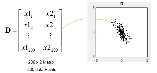
In this application, I will use SVD to find the principal components for a data set. Principal components means the axis (a vector) that represents the direction along which the data is most widely distributed, i.e the axis with the largest variance. In this example, I will use a 200 x 2 matrix which represents the 200 data points as plotted below.
First I assinged the D matrix to Matrix M. There is no mathmatical reason to do this. I just did this because I wanted to use the matrix M for all the matlab examples for this page.
![]()
Then I did SVD as follows.
![]()
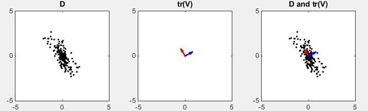
D in the following plots represents the data set in scatter plot. You would intuitively find an axis along which the data are spread most widely. tr(V) shows two row vectors in transpose(V) vector that came from SVD. You see the red arrow is pointing the princial components, i.e the major axis. The third plot shows the transpose(V) vectors overlayed onto the data set. (Matlab source code for this example is in < List 1 >)
|
|
|||
| The result of SVD is as follows. | |||
|
M = D (data points) |
U |
S |
transpose(V) |
|
200 x 2 Matrix (Data Points) |
200 x 200 Matrix |
200 x 2 Matrix ------------------------ 14.6873 0 0 4.9745 . . all zeros . |
-0.4940 0.8695 0.8695 0.4940 |
In this example, I defined the M matrix as follows. (The covariance matrix of the data set is assinged to M. Now M is 2 x 2 square matrix)
![]()
Then I did SVD as follows.
![]()
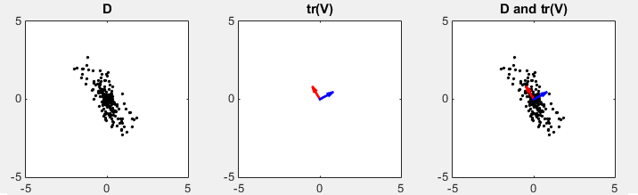
D in the following plots represents the data set in scatter plot. You would intuitively find an axis along which the data are spread most widely. tr(V) shows two row vectors in transpose(V) vector that came from SVD. You see the red arrow is pointing the princial components, i.e the major axis. The third plot shows the transpose(V) vectors overlayed onto the data set. (Matlab source code for this example is in < List 2 >)
|
|
|||
| Following is the result of SVD. You see that transpose(V) is same as the first example. S (eigen value) shows different value. It means the principal axis is same as in previous method. | |||
|
M = tr(D).D |
U |
S |
transpose(V) |
|
71.3471 -82.0238 -82.0238 169.1167 |
-0.4940 0.8695 0.8695 0.4940 |
215.7181 0 0 24.7457 |
-0.4940 0.8695 0.8695 0.4940 |
In this example, I defined the M matrix as follows. (The covariance matrix of the data set is assinged to M. Now M is 2 x 2 square matrix)
![]()
Then I calculated the eigenvector and eigen value.
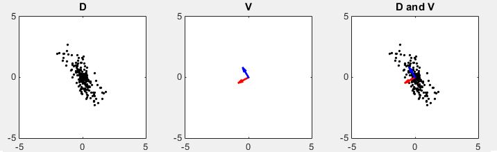
D in the following plots represents the data set in scatter plot. You would intuitively find an axis along which the data are spread most widely. V shows two eigen vectors. Even though the color of the vector are swapped comparing to previous method, the direction of two arrows are still same. (Matlab source code for this example is in < List 3 >)
|
|
|||
|
Following is the result of Eigenvalue and Eigenvalues. In case of SVD, the basis vector (vectors in V matrix) is arranged in decreasing order of the corresponding eigenvalues, but eigenvalue calculation does not follows this kind of ordering. |
|||
|
M = tr(D).D |
V(Eigenvector) |
E (Eigenvalues) |
|
|
71.3471 -82.0238 -82.0238 169.1167 |
-0.8695 -0.4940 -0.4940 0.8695 |
24.7457 0 0 215.7181 |
|
< List 1 >
clear all;
N = 200;
rng(1);
t = rand(1,N);
rng(1);
r = randn(1,N);
x1 = 0.5 .* r .* cos(2*pi*t);
x2 =1.5 .* r .* sin(2*pi*t);
M = [x1; x2];
tm = [cos(pi/6) -sin(pi/6);sin(pi/6) cos(pi/6)]
D = (tm * M)';
x = D(:,1);
y = D(:,2);
M = D;
[U,S,V]=svd(M);
vT = V';
vT1 = vT(1,:);
vT2 = vT(2,:);
sigma1 = S(1,1);
sigma2 = S(2,2);
subplot(1,3,1);
plot(x,y,'ko','MarkerFaceColor',[0 0 0],'MarkerSize',2);
axis([-5 5 -5 5]);
title('D');
subplot(1,3,2);
quiver(0,0,vT1(1),vT1(2),'r','MaxHeadSize',1.5,'linewidth',2);
axis([-5 5 -5 5]);
hold on;
quiver(0,0,vT2(1),vT2(2),'b','MaxHeadSize',1.5,'linewidth',2);
axis([-5 5 -5 5]);
hold off;
title('tr(V)');
subplot(1,3,3);
plot(x,y,'ko','MarkerFaceColor',[0 0 0],'MarkerSize',2);
axis([-5 5 -5 5]);
hold on;
quiver(0,0,vT1(1),vT1(2),'r','MaxHeadSize',1.5,'linewidth',2);
axis([-5 5 -5 5]);
hold on;
quiver(0,0,vT2(1),vT2(2),'b','MaxHeadSize',1.5,'linewidth',2);
axis([-5 5 -5 5]);
hold off;
title('D and tr(V)');
< List 2 >
clear all;
N = 200;
rng(1);
t = rand(1,N);
rng(1);
r = randn(1,N);
x1 = 0.5 .* r .* cos(2*pi*t);
x2 =1.5 .* r .* sin(2*pi*t);
M = [x1; x2];
tm = [cos(pi/6) -sin(pi/6);sin(pi/6) cos(pi/6)]
D = (tm * M)';
x = D(:,1);
y = D(:,2);
M = D' * D;
[U,S,V]=svd(M);
vT = V';
vT1 = vT(1,:);
vT2 = vT(2,:);
sigma1 = S(1,1);
sigma2 = S(2,2);
subplot(1,3,1);
plot(x,y,'ko','MarkerFaceColor',[0 0 0],'MarkerSize',2);
axis([-5 5 -5 5]);
title('D');
subplot(1,3,2);
quiver(0,0,vT1(1),vT1(2),'r','MaxHeadSize',1.5,'linewidth',2);
axis([-5 5 -5 5]);
hold on;
quiver(0,0,vT2(1),vT2(2),'b','MaxHeadSize',1.5,'linewidth',2);
axis([-5 5 -5 5]);
hold off;
title('tr(V)');
subplot(1,3,3);
plot(x,y,'ko','MarkerFaceColor',[0 0 0],'MarkerSize',2);
axis([-5 5 -5 5]);
hold on;
quiver(0,0,vT1(1),vT1(2),'r','MaxHeadSize',1.5,'linewidth',2);
axis([-5 5 -5 5]);
hold on;
quiver(0,0,vT2(1),vT2(2),'b','MaxHeadSize',1.5,'linewidth',2);
axis([-5 5 -5 5]);
hold off;
title('D and tr(V)');
< List 3 >
clear all;
N = 200;
rng(1);
t = rand(1,N);
rng(1);
r = randn(1,N);
x1 = 0.5 .* r .* cos(2*pi*t);
x2 =1.5 .* r .* sin(2*pi*t);
M = [x1; x2];
tm = [cos(pi/6) -sin(pi/6);sin(pi/6) cos(pi/6)]
D = (tm * M)';
x = D(:,1);
y = D(:,2);
M = D' * D;
[V,E] = eig(M);
vT = V;
vT1 = vT(:,1);
vT2 = vT(:,2);
sigma1 = E(1,1);
sigma2 = E(2,2);
subplot(1,3,1);
plot(x,y,'ko','MarkerFaceColor',[0 0 0],'MarkerSize',2);
axis([-5 5 -5 5]);
title('D');
subplot(1,3,2);
quiver(0,0,vT1(1),vT1(2),'r','MaxHeadSize',1.5,'linewidth',2);
axis([-5 5 -5 5]);
hold on;
quiver(0,0,vT2(1),vT2(2),'b','MaxHeadSize',1.5,'linewidth',2);
axis([-5 5 -5 5]);
hold off;
title('V');
subplot(1,3,3);
plot(x,y,'ko','MarkerFaceColor',[0 0 0],'MarkerSize',2);
axis([-5 5 -5 5]);
hold on;
quiver(0,0,vT1(1),vT1(2),'r','MaxHeadSize',1.5,'linewidth',2);
axis([-5 5 -5 5]);
hold on;
quiver(0,0,vT2(1),vT2(2),'b','MaxHeadSize',1.5,'linewidth',2);
axis([-5 5 -5 5]);
hold off;
title('D and V');
Reference :
[1] Principal Component Analysis (PCA) - YouTube
[2] StatQuest: Principal Component Analysis (PCA), Step-by-Step - YouTube