Every feature before this one made a single cell work harder. CoMP does something else: it asks several transmission points to act as one for a UE that can hear more than one of them. What follows is why that helps, the deployments 3GPP wrote it for, the shapes the coordination can take, and the RRC machinery that carries it.
- Why CoMP ?
- Proposed Scenarios
- Homogenous Network vs Heterogenous Network
- CoMP Categories
- CoMP Sets
- RRC Aspect of CoMP
- Videos :
- Reference :
Why CoMP ?
As you may learned from the evolution path of any wireless communication, the strongest motivation for new technology and new feature is to increase the throughput and/or to increase the reliability of the communication. Some features are more focused on the reliability issues and some features would be more focused on throughput issues.
Let's take a high level view of several LTE features of LTE in terms of the two aspects, reliability and throughput. As you can naturally think, LTE development started with SISO configuration (I think this was only in development stage, by the time LTE started being deployed everything was 2 x 2 MIMI by default) and the technology evolved to MIMO. Definately this is mainly for increasing the throughput. Since the initial LTE deployment, 2 x 2 MIMO has been the dominent feagure for most of LTE device and LTE network. Then another evolution for throughput improvement started being adopted. It was Carrier Aggregation (mainly Carrier Aggregation between two different bands).
Once the throughput evolution by Carrier Aggregation is implemented, another path of evolution is being discussed. This new evolution path also eventually lead to throughput improvement, but direct effect of this evolution would be to increase spectral efficiency especially in cell-edge area and decrease interference between multiple cells by letting UE communicate with multiple cells in specially coordinated manner. This new technology is called CoMP (Coordinated multi-point operation).
The motivation of CoMP officially described by 3GPP are
- to improve the coverage of high data rate
- to improve the cell-edge throughput
- to increase the system throughput (See following 'Note').
Note : I just learned (after discussion with expert engineer in this area) that the CoMP does not support special Multiplexing between TPs, so there would be no increase of the throughput in terms of Max throughput on UE side.
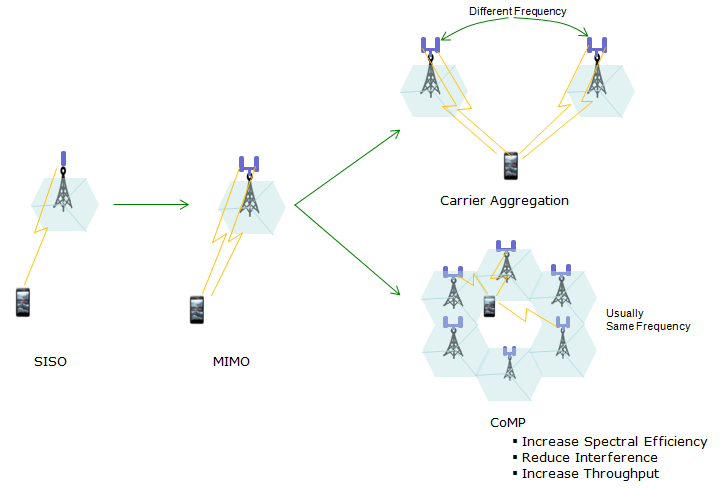
The split at the right of the drawing is the point. Carrier aggregation adds a second frequency, and CoMP stays on one frequency and adds a second point instead.
The left half is the single cell story : SISO, then MIMO, both drawn against one base station.The upper branch adds a frequency : two sites marked Different Frequency, which is carrier aggregation.The lower branch adds points : six cells around one UE, marked Usually Same Frequency.The gains listed under CoMP are three : Increase Spectral Efficiency, Reduce Interference and Increase Throughput.
Proposed Scenarios
According to 3GPP TR 36.819 V11.2.0 (2013-09), 4 different scenario were proposed for the situations where CoMP can be benificial and these fource scenarios are illustrated as shown below.

Three panels cover four scenarios. Scenarios 3 and 4 share the last one because they differ only in whether the remote radio heads carry their own cell identity, and a drawing cannot show a cell identity.
Following is brief description of each scenario
< Scenario 1 >
- Applies to Homogeneous network (No optical fiber backhaul connection is needed)
- Intra-site CoMP : Coordination between the cells (sectors) controlled by the same macro base station
< Scenario 2 >
- Applies to Homogeneous network
- CoMP between a Macro cell and multiple high Tx power RRH (Remote Radio Head)
< Scenario 3 >
- Applies to Heterogeneous network
- CoMP between a Macro cell and multiple low Tx power RRH (Remote Radio Head)
- Transmission/Reception points created by RRH have different cell ID from the Macro Cell's ID
< Scenario 4 >
- Applies to Heterogeneous network
- CoMP between a Macro cell and multiple low Tx power RRH (Remote Radio Head)
- Transmission/Reception points created by RRH have same cell ID as the Macro Cell's ID
The optical fibre drawn in the second and third panels is the part that matters. Coordination needs the points to exchange channel state information, and in the first panel they do not need a link at all because the sectors already sit in one base station. That is the difference the scenario list calls intra-site.
Cell identity separates scenario 3 from scenario 4, and it decides what the UE believes it is looking at. With separate identities the remote radio heads are cells the UE can measure and report on their own. With a shared identity they are not, and the coordination has to be invisible to the measurement machinery.
Scenario 1 needs no backhaul link : the coordinated sectors already belong to one macro base station.Scenarios 2, 3 and 4 need one : the panels draw it as optical fibre between the macro and the remote radio heads.Transmit power separates 2 from 3 and 4 : high power remote radio heads in one, low power in the others.Cell identity separates 3 from 4 : different identities in scenario 3, the macro's own identity in scenario 4.
Homogenous Network vs Heterogenous Network
The two words appear in every CoMP scenario list, and the scenarios split along the line between them. The difference is not size or vendor but transmit power, and it decides how much interference reaches a UE at the edge of a cell.
Homogenous Network : a network composed of all the base stations belong to the same type and power class.
Heterogenous Network : a network composed of different base station type and different power classes. This type of network may be exposed to harsh intercell interference between the macro and the low-power nodes, due to their closer proximity and different power classes.
The distinction decides which scenario a deployment falls into. A homogenous network covers scenario 1 and scenario 2, because every point transmits at a comparable power. A heterogenous network is what scenario 3 and scenario 4 describe, where a low power point sits inside the coverage of a high power one.
Interference is the reason the second case is harder. A UE near a low power point still hears the macro at a much stronger level. The useful signal and the interference therefore arrive from different directions and at very different powers, and CoMP coordinates the two rather than making either of them stronger.
Homogenous means one power class : every base station in the network is the same type.Heterogenous means several : a low power point sits inside the coverage of a high power one.The scenarios split along that line : 1 and 2 are homogenous, 3 and 4 are heterogenous.The hard case is the mixed one : signal and interference arrive at very different powers.
CoMP Categories
The schemes differ in one thing only, which is how much the coordinating points share. Sharing channel state information alone is the cheapest arrangement, and sharing the user data as well is the most expensive. The tree below sorts every named scheme along that line.

The tree has more in it than the notes below it cover. Downlink CoMP splits into coordinated scheduling and joint processing, and joint processing divides again into joint transmission and dynamic point selection.
Joint Processing is the parent term : both joint transmission and dynamic point selection sit under it in the drawing.Joint Transmission divides again : Coherent JT and Non-Coherent JT, which is whether the points align their phase.Dynamic Point Selection divides too : With Muting and Without Muting, which is whether the points that are not chosen stay silent.The uplink branch is shorter : coordinated scheduling and beamforming again, and Joint Reception in place of joint transmission.The drawing says DPS where the notes say TPS : the third downlink scheme is labelled Dynamic Point Selection in the tree and Transmission Point Selection in the heading under it.
< CS/CB (Coordinated Scheduling/Coordinated Beamforming) >
- Multiple coordinated TP (Transmission Points) shares only CSI for multiple UEs and data packet that is destined to a specific UE is available only at one TP.
- In CB, power level and the beamforming coefficients are calculated to achieve some common SINRs in the system or to maximize the minimum SNIR.
- In CS, a network is divided into multiple clusters and apply centeralized scheduling within each cluster in order to determine which TPs in the cluster should transmit in each time slot and to which UE.
- CS/CB is a technology that jointly use CB and CS.
< JT (Joint Transmission) >
- Multiple Coordinated TPs are transmitting the same data with appropriate Beamforming weights

< TPS (Transmission Point Selection) >
- It can be regarded as a special form of JT.
- Transmission of beamformed data for a given UE terminal is performed at a single TP at each time instance
- This technique enables UE to be dynamically scheduled by the best TP by exploiting changes in the channel fading condition.

The two drawings above are best read as a pair. In the joint transmission one, both points send a data arrow to the same UE and a central processing block holds the data as well as the CSI. In the selection one, the same picture is drawn twice and only one point sends the data arrow in each copy, with a dashed arrow underneath saying the state changes dynamically.
That is the cost difference in one image. Joint transmission needs the user data at every participating point before the subframe is sent. Dynamic point selection needs the data at one point, and the coordination decides which one. Coordinated scheduling and beamforming needs no user data to be shared at all.
CS/CB shares channel state information only : the data for a UE stays at the point that serves it.Joint transmission shares the data too : every participating point must hold it before the subframe goes out.Dynamic point selection shares data but uses one point : the choice of point changes from subframe to subframe.Muting is the variant worth knowing : the points that are not chosen can be told to stay silent rather than transmit to somebody else.Joint Reception is the uplink counterpart : several points receive one UE, and the drawing puts it opposite joint processing.
CoMP Sets
As the name (CoMP : Coordinated Mult-Point) implies, CoMP is operating in the unit of multiple points. This multiple points participating in CoMP is called a 'Set'. There are two large categories of CoMP Sets as described below.
< CoMP Operating Set >
CoMP Operating Set is a multiple geographically separated points participating in CoMP operation.
- Each points within a set can either directly or indirectly participates in CoMP operation.
- Direct participation means that those points actually transmit data
- Indirect participation means that those points does not transmit data but influence on CoMP operation by contributing in making decisions on the user scheduling/beamforming
- CoMP Transmission point(s) within a set may work in a little different way depending on CoMP scheme(Category)
- In JT (Joint Transmission), all of these points would transmit data at the scheduled subframe
- In CS/CB, DPS, SSPS, only one of these points actually transmit data and other points assists with CoMP operation
< CoMP Measurement Set >
CoMP measurement set is a multiple geographically separated points about which a UE perform measurement (CSI) and report the result.
The two sets answer different questions, and the difference matters when a log is being read. The operating set is a network side idea about which points take part. The measurement set is a UE side idea about which points the UE is told to measure and report.
Neither set is signalled to the UE under that name. 36.331 carries the measurement set as a list of CSI processes, and each process names one channel measurement resource and one interference measurement resource. The section below reads that structure.
The operating set is about transmission : which points take part, directly or indirectly.The measurement set is about reporting : which points the UE measures and reports CSI for.Indirect participation still counts : a point that sends no data can still contribute to the scheduling decision.The scheme decides how many points transmit : all of them under joint transmission, one of them under CS/CB and dynamic point selection.Neither name appears in RRC : the measurement set reaches the UE as a list of CSI processes.
RRC Aspect of CoMP
Following is the overall structure of RRC Message information elements related to CoMP. This is just summary and I think it will take several month for me to come up with all the details. As of now (Feb 2015), I haven't seen any chipset that support CoMP and I think it will take at least several month before we hear of the chipset supporting this feature. I will keep updating the details as I learn further.


csi-IM-ConfigToAddModList : For a serving frequency E-UTRAN configures one or more CSI-IM-Config only when transmission mode 10 is configured for the serving cell on this carrier frequency.
csi-ProcessToAddModList : For a serving frequency E-UTRAN configures one or more CSI-Process only when transmission mode 10 is configured for the serving cell on this carrier frequency.
resourceConfig : CSI reference signal configuration, see TS 36.213 7.2.6 and TS 36.211 table 6.10.5.2-1 and 6.10.5.2-2] for 4 REs.
< TS 36.211 - Table 6.10.5.2-1: Mapping from CSI reference signal configuration to (k', l' ) for normal cyclic prefix >

subframeConfig : I_CSI−RS
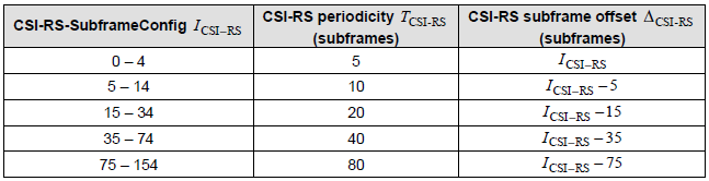
< 36.211 - Table 6.10.5.3-1: CSI reference signal subframe configuration >
One transmission mode gates the whole of it. 36.331 attaches the same condition to field after field: E-UTRAN configures one or more CSI-IM-Config only when transmission mode 10 is configured, and the same wording governs CSI-Process, CSI-RS-ConfigZP and pdsch-ConfigDedicated-v1130. One field is the reverse case, and csi-RS-Config is the one E-UTRAN does not configure under transmission mode 10.
A CSI process is the structure that makes CoMP reporting work. 36.331 gives CSI-Process-r11 a csi-RS-ConfigNZPId and a csi-IM-ConfigId, so one process pairs the resource the UE measures the wanted signal on with the resource it measures interference on. A report per process is how a UE says what each candidate point would give it.
The counts are small and worth remembering. 36.331 sets maxCSI-Proc-r11 to 4, so a carrier carries at most four CSI processes. It sets maxCSI-IM-r11 to 3 in Release 11, later raised to 4 and then to 24. It sets maxRE-MapQCL-r11 to 4, which is the annotation the decode above carries beside its RE mapping list.
The two 36.211 tables below turn one configured number into a position and a schedule. Table 6.10.5.2-1 maps the CSI reference signal configuration onto a subcarrier and symbol pair, . Fewer columns are filled as the port count rises, because eight ports consume more resource elements than two. Table 6.10.5.3-1 maps the subframe configuration index onto both a periodicity and an offset, so 0 to 4 means every 5 subframes and 75 to 154 means every 80.
Transmission mode 10 is the gate : 36.331 conditions the CoMP fields on it, one field at a time.csi-RS-Config is the exception : E-UTRAN does not configure it when transmission mode 10 is in use.A CSI process pairs two resources : csi-RS-ConfigNZPId for the signal and csi-IM-ConfigId for the interference.Four processes per carrier : 36.331 sets maxCSI-Proc-r11 to 4, and maxRE-MapQCL-r11 to 4 as well.One index carries period and offset : 36.211 Table 6.10.5.3-1 splits the CSI-RS subframe configuration into both.
Videos :
Reference :
[1] 3GPP TR 36.819 V11.2.0 (2013-09)
[2] 3GPP TS 36.211
[3] IEEE Communications Magazine • February 2012 : Coordinated Multipoint Transmission and Reception in LTE-Advanced: Deployment Scenarios and Operational Challenges by
Daewon Lee and Hanbyul Seo, LG Electronics
Bruno Clerckx, Samsung Electronics
Eric Hardouin, Orange Labs
David Mazzarese, Huawei Technologies
Satoshi Nagata, NTT DOCOMO
Krishna Sayana, Motorola Mobility
[4] 36.331 : 3GPP - E-UTRA; Radio Resource Control, v19.3.0. CSI-Process-r11 pairs a CSI-RS resource with an interference measurement resource, and the transmission mode 10 conditions on the CoMP fields are in the field descriptions.
[5] 36.211 : 3GPP - E-UTRA; Physical channels and modulation, v19.3.0. Table 6.10.5.2-1 and Table 6.10.5.3-1 are the two tables shown above, and both still read as the screenshots show them.