What I am going to do is basically same as what I did with a multi layer perceptron example. Then why do I want to do it again ? As might have noticed in perceptron example, the coding gets more and more complicated as the number of layers increases and the number of neurons increases mainly due to the initialization and layer connection configuration. In this example, I will show you a simpler way to do the same thing as we did with perceptron network.
You may ask why I even tried the same thing in more complicated way with perceptron while you have simpler way to do it. I have a good reason for it. Usually when there are multiple ways to do the same thing, simple vs complicated one, complicated one tend to show more details on how it works whereas simpler version tend to automate many things and hide the internal complexity. So if you want to know more details on how the common network (especially fully forward connected network), I would suggest you to go through all the examples with perceptron network from single perceptron through multi layer/multi neuron networks.
In short, the main purpose of this tutorial is to introduce a feedforwardnet() function in Matlab ML toolbox. I would not redo the very simple case like 1 perceptron or the hidden layer with too small number of neurons since for those simple case feedforwardnet() would not give you much advantange. I will start with 7 neurons in the hidden layer case and then jump to 30 neurons in the hidden layer case just to show you that how simple it is to build a network using feedforwardnet() regardless of the number of neurons in each layers.
Hidden Layer : 7 nuerons in Hiddel Layer, 1 Output
In this example, I will try to classify this data using two layer network : 7 perceptrons in the Hidden layer and one output perceptron. Let's see how well this work.
The basic logic is exactly same as in previous section. The only difference is that I have more cell(perceptron) in the hidden layer.
What do you think ? Would it give a better result ?
If it give poorer result, would it be because of this one additional cell in the hidden layer ? or would it be because other training parameters are not optimized properly.
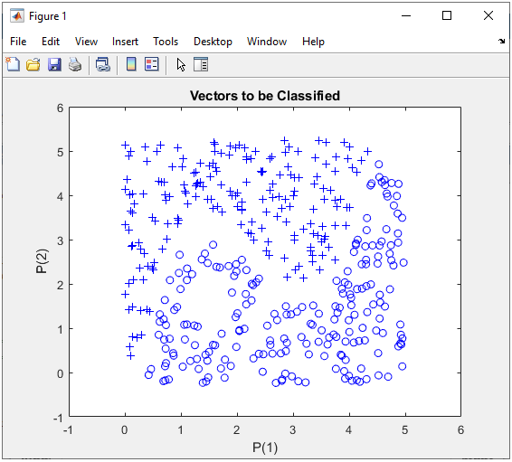
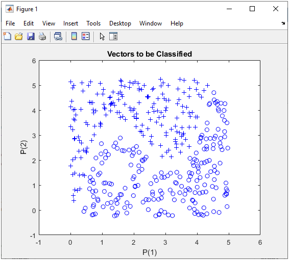
Step 1 : Take a overall distribution of the data plotted as below and try to come up with some idea what kind of neural network you can use. I use the following code to create this dataset. It would not be that difficult to understand the characteristics of dataset from the code itself, but don't spend too much time and effort to understand this part. Just use it as it is.
full_data = [];
xrange = 5;
for i = 1:400
x = xrange * rand(1,1);
y = xrange * rand(1,1);
if y >= 0.6 * (x-1)*(x-2)*(x-4) + 3
y = y + 0.25;
z = 1;
else
y = y - 0.25;
z = 0;
end
full_data = [full_data ; [x y z]];
end
In this case, only two parameters are required to specify a specific data. That's why you can plot the dataset in 2D graph. Of course, in real life situation this would not be a frequent case where you can have this kind of simple dataset, but I would recommend you to try with this type of simple dataset with multiple variations and understand exactly what type of variation you have to make in terms of neural network structure to cope with those variations in data set.
Step 2 : Determine the structure of Neural Nework.
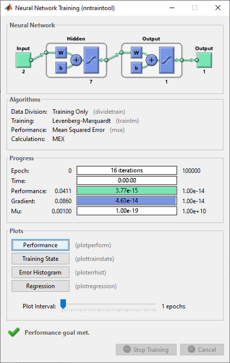
As mentioned above, the purpose of this experiement is to see how the network works when I add more cells in the hidden layer. So the structure should look as follows.

This structure can be created by following code. Compare this with perceptron network case for the same network shown here and see how simpler it is to use feedforwardnet() function. Basically it is just one line of code to create the network and additional lines after feedforwardnet() is to change some parameters. If you want to use the default parameters, you don't need to add those additional lines.
net = feedforwardnet(7); % NOTE : the number 7 here indicate the number of neurons in the first layer
% (i.e, the hidden layer in the whole network). You don't need to specify Output
% layer because it is automatically set by the output data you are poassing in
% train() function.
net.performFcn = 'mse';
net.trainFcn = 'trainlm';
net.divideFcn = 'dividetrain';
net.layers{1}.transferFcn = 'tansig';
net.layers{2}.transferFcn = 'tansig';
Step 3 : Train the network.
Training a network is done by a single line of code as follows.
[net,tr] = train(net,pList,tList);
Just running this single line of code may nor may not solve your problem. In that case, you may need to tweak the parameters involved in the training process. First tweak the following parameters and try with different activation functions in step 2.
net.trainParam.epochs =100000;
net.trainParam.goal = 10^-14;
net.trainParam.min_grad = 10^-14;
net.trainParam.max_fail = 1000;
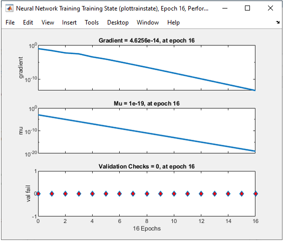
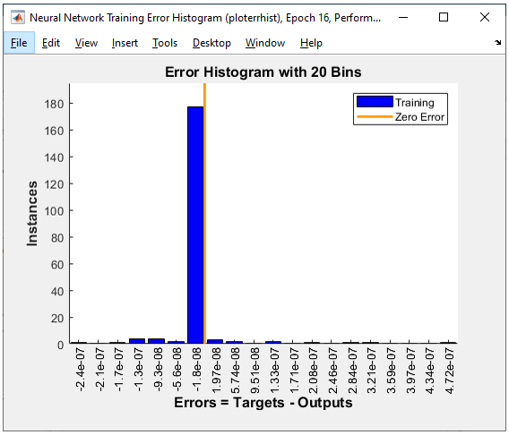
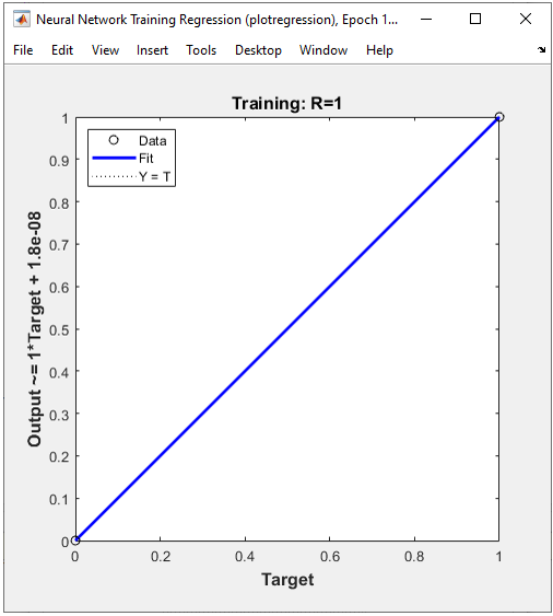
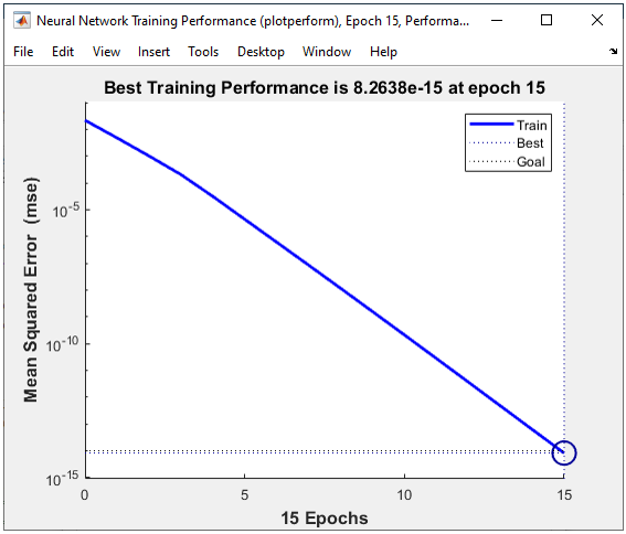
The result in this example is as shown below.
As shown below, the performance is similar to the perceptron network with the same same number of neurons in each layer.
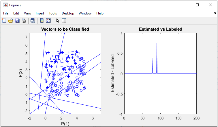
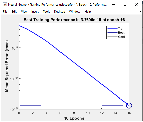
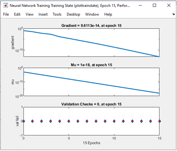
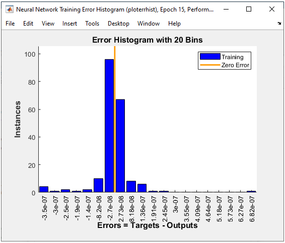
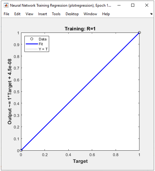
All of the following plots are showing how the training process reaches the target at each iteration. I would not explain on these plots.
|
% Generate Data Set rng(1); full_data = [];
xrange = 5; for i = 1:400
x = xrange * rand(1,1); y = xrange * rand(1,1);
if y >= 0.6 * (x-1)*(x-2)*(x-4) + 3 y = y + 0.25; z = 1; else y = y - 0.25; z = 0; end
full_data = [full_data ; [x y z]];
end
% Split the dataset into Training set and Test Set data_Train = full_data(1:200,:); data_Test = full_data(201:400,:);
% Initialize Input Vector with Training Dataset pList = [data_Train(:,1)'; data_Train(:,2)']; tList = data_Train(:,3)';
figure(1); plotpv([full_data(:,1)'; full_data(:,2)'],full_data(:,3)'); axis([-1 6 -1 6]);
figure(2); set(gcf, 'Position', [100, 100, 750, 350]);
% Build a Neural Net subplot(1,2,1);
plotpv(pList,tList);
net = feedforwardnet(7);
net.performFcn = 'mse'; net.trainFcn = 'trainlm'; net.divideFcn = 'dividetrain';
net.layers{1}.transferFcn = 'tansig'; net.layers{2}.transferFcn = 'tansig';
% Perform Training
net.trainParam.epochs =100000; net.trainParam.goal = 10^-14; net.trainParam.min_grad = 10^-14; net.trainParam.max_fail = 1000;
view(net);
[net,tr] = train(net,pList,tList);
% Plot Training Result
for i = 1:length(net.iw{1,1}) plotpc(net.iw{1,1}(i,:),net.b{1}(i,:)); hold on end
pList = [data_Test(:,1)'; data_Test(:,2)']; tList = data_Test(:,3)';
subplot(1,2,2);
y = net(pList); plot(y-tList,'b-'); ylim([-1 1]); ylabel('Estimated - Labeled'); title('Estimated vs Labeled'); |
Hidden Layer : 30 nuerons in Hiddel Layer, 1 Output
The problem that I want to solve in this example is same as what I did with perceptron, but the complexity of the network in this exaample hasn't been tried in perceptron net becaues it would have been too complicated for perceptron net. I am going to put 30 neurons in the hidden layer which is much larger comparing to what I used in perceptron example.
You may have some questions as follows before you jump into writing the code.
- You have increased the number of neurons in the Hidden layer drastically, will it give you the drastically increased performance ?
- How about the complexity of the code ? Will it be much more complicated comparing to the case with less number of neurons in Hidden Layer ?
You will find the answers soon.
Step 1 : Take a overall distribution of the data plotted as below and try to come up with some idea what kind of neural network you can use. I use the following code to create this dataset. It would not be that difficult to understand the characteristics of dataset from the code itself, but don't spend too much time and effort to understand this part. Just use it as it is.
full_data = [];
xrange = 5;
for i = 1:400
x = xrange * rand(1,1);
y = xrange * rand(1,1);
if y >= 0.6 * (x-1)*(x-2)*(x-4) + 3
y = y + 0.25;
z = 1;
else
y = y - 0.25;
z = 0;
end
full_data = [full_data ; [x y z]];
end
In this case, only two parameters are required to specify a specific data. That's why you can plot the dataset in 2D graph. Of course, in real life situation this would not be a frequent case where you can have this kind of simple dataset, but I would recommend you to try with this type of simple dataset with multiple variations and understand exactly what type of variation you have to make in terms of neural network structure to cope with those variations in data set.
Step 2 : Determine the structure of Neural Nework.
As mentioned above, the purpose of this experiement is to see how the network works when I add more cells in the hidden layer. So the structure should look as follows.
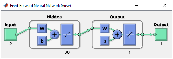
This structure can be created by following code. Compare this with perceptron network case for the same network shown here and see how simpler it is to use feedforwardnet() function. Basically it is just one line of code to create the network and additional lines after feedforwardnet() is to change some parameters. If you want to use the default parameters, you don't need to add those additional lines.
net = feedforwardnet(30); % NOTE : This is the only difference between this example and previous example.
% NOTE : the number 30 here indicate the number of neurons in the first layer
% (i.e, the hidden layer in the whole network). You don't need to specify Output
% layer because it is automatically set by the output data you are poassing in
% train() function.
net.performFcn = 'mse';
net.trainFcn = 'trainlm';
net.divideFcn = 'dividetrain';
net.layers{1}.transferFcn = 'tansig';
net.layers{2}.transferFcn = 'tansig';
Step 3 : Train the network.
Training a network is done by a single line of code as follows.
[net,tr] = train(net,pList,tList);
Just running this single line of code may nor may not solve your problem. In that case, you may need to tweak the parameters involved in the training process. First tweak the following parameters and try with different activation functions in step 2.
net.trainParam.epochs =100000;
net.trainParam.goal = 10^-14;
net.trainParam.min_grad = 10^-14;
net.trainParam.max_fail = 1000;
The result in this example is as shown below.
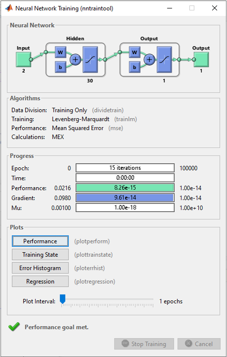
The result is as shown below. I see just a little bit of improvement comparing to previous example (i.e, 7 neurons in Hidden Layer), but not so confident whether it is worth increasing this many of neurons for this problem which requires much more computational power.
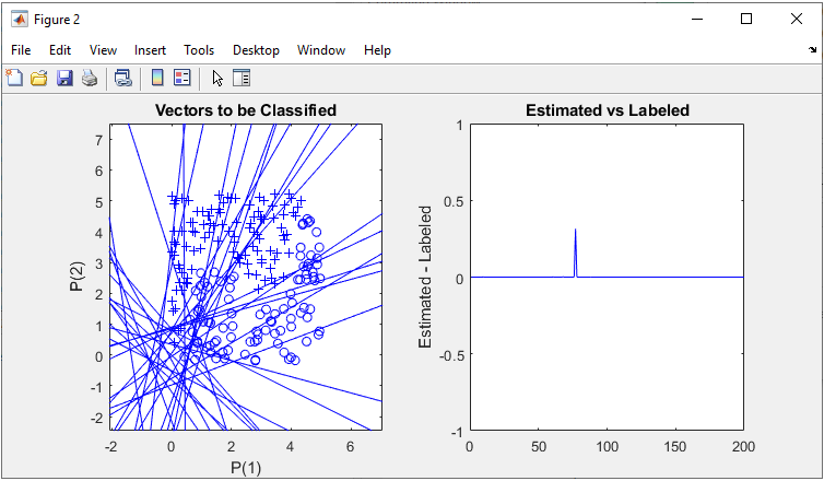
As shown below, the performance is similar to the perceptron network with the same same number of neurons in each layer.
|
% Generate Data Set rng(1); full_data = [];
xrange = 5; for i = 1:400
x = xrange * rand(1,1); y = xrange * rand(1,1);
if y >= 0.6 * (x-1)*(x-2)*(x-4) + 3 y = y + 0.25; z = 1; else y = y - 0.25; z = 0; end
full_data = [full_data ; [x y z]];
end
% Split the dataset into Training set and Test Set
data_Train = full_data(1:200,:); data_Test = full_data(201:400,:);
% Initialize Input Vector with Training Dataset pList = [data_Train(:,1)'; data_Train(:,2)']; tList = data_Train(:,3)';
figure(1); plotpv([full_data(:,1)'; full_data(:,2)'],full_data(:,3)'); axis([-1 6 -1 6]);
figure(2); set(gcf, 'Position', [100, 100, 750, 350]);
% Build a Neural Net
subplot(1,2,1);
plotpv(pList,tList);
net = feedforwardnet(30);
net.performFcn = 'mse'; net.trainFcn = 'trainlm'; net.divideFcn = 'dividetrain';
net.layers{1}.transferFcn = 'tansig'; net.layers{2}.transferFcn = 'tansig';
% Perform Training
net.trainParam.epochs =100000; net.trainParam.goal = 10^-14; net.trainParam.min_grad = 10^-14; net.trainParam.max_fail = 1000;
view(net);
[net,tr] = train(net,pList,tList);
% Plot Training Result for i = 1:length(net.iw{1,1}) plotpc(net.iw{1,1}(i,:),net.b{1}(i,:)); hold on end
pList = [data_Test(:,1)'; data_Test(:,2)']; tList = data_Test(:,3)';
subplot(1,2,2);
y = net(pList); plot(y-tList,'b-'); ylim([-1 1]); ylabel('Estimated - Labeled'); title('Estimated vs Labeled'); |
Next Step :