|
SciPy - Basics
SciPy (Scientific Python) is an open-source Python library used for scientific and technical computing. It is built on top of the NumPy library and provides additional functionality for working with arrays and numerical data. SciPy extends NumPy's capabilities by offering a wide range of algorithms and tools for different scientific domains.
The key features of the SciPy library are:
Integration: SciPy provides functions for numerical integration, such as single, double, and triple integrals, as well as for solving ordinary differential equations (ODEs).
Optimization: The library contains optimization algorithms for finding minima or maxima of functions, curve fitting, root finding, and linear programming. These algorithms can be applied to various optimization problems in engineering, physics, and other scientific fields.
Interpolation: SciPy offers interpolation functions for one-dimensional and multi-dimensional data, allowing users to fit smooth curves to given data points.
Signal Processing: SciPy provides signal processing tools for filtering, convolution, spectral analysis, and window functions. These tools are commonly used in applications such as image and audio processing, communication systems, and control systems.
Linear Algebra: The library includes a comprehensive set of linear algebra functions, such as matrix operations, eigenvalue and eigenvector computations, and various factorizations and decompositions. These functions are essential for many scientific and engineering applications.
Statistics: SciPy includes a rich set of statistical functions for probability distributions, summary statistics, hypothesis testing, and more. This functionality is useful in data analysis, machine learning, and other statistical applications.
Spatial: The library offers spatial algorithms and data structures for working with geometrical objects, such as points, lines, polygons, and more. It also provides tools for spatial data analysis, such as distance computations, nearest-neighbor searches, and clustering.
Image Processing: SciPy includes image processing functions for image filtering, morphology, transformations, and other image manipulation tasks. These functions are used in various computer vision and image analysis applications.
File I/O: The library supports reading and writing data to various file formats, such as NetCDF, MATLAB, and others, which is essential for interoperability with other scientific software.
Importing the package
you can import a specific subpackage you want to use as shown below
|
import numpy as np
import matplotlib.pyplot as plt
from scipy.fftpack import fft
t = np.linspace(0,10*np.pi,100);
sig = np.cos(3*t);
sig_freq = fft(sig);
plt.plot(t,sig_freq,'r-');
plt.show();
|
or you can import the full package as shown below.
|
import numpy as np
import matplotlib.pyplot as plt
import scipy as sp
t = np.linspace(0,10*np.pi,100);
sig = np.cos(3*t);
sig_freq = sp.fft(sig);
plt.plot(t,sig_freq,'r-');
plt.show();
|
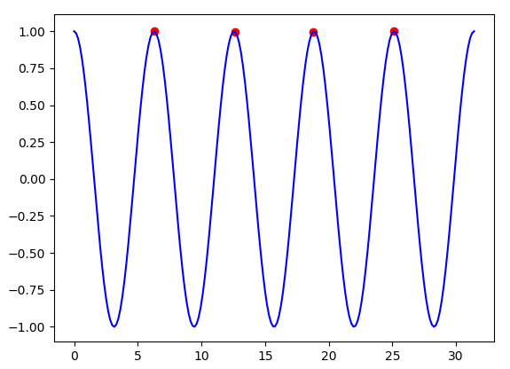
Finding Peaks
< Find all the peaks >
|
import numpy as np
import matplotlib.pyplot as plt
import scipy as sp
from scipy.signal import find_peaks
t = np.linspace(0,10*np.pi,200);
x = np.cos(t);
peaks,_ = find_peaks(x);
plt.plot(t, x,'b-');
plt.scatter(t[peaks],x[peaks],c='red');
plt.show();
|
|
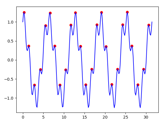
import numpy as np
import matplotlib.pyplot as plt
import scipy as sp
from scipy.signal import find_peaks
t = np.linspace(0,10*np.pi,200);
x = np.cos(t) + 0.3*np.sin(5*t);
peaks,_ = find_peaks(x);
plt.plot(t, x,'b-');
plt.scatter(t[peaks],x[peaks],c='red');
plt.show();
|
< Find the peaks above a threshold >
|
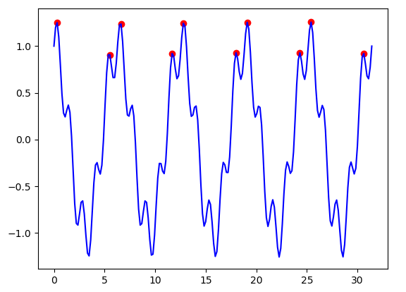
import numpy as np
import matplotlib.pyplot as plt
import scipy as sp
from scipy.signal import find_peaks
t = np.linspace(0,10*np.pi,200);
x = np.cos(t) + 0.3*np.sin(5*t);
peaks,_ = find_peaks(x, height = 0.5);
plt.plot(t, x,'b-');
plt.scatter(t[peaks],x[peaks],c='red');
plt.show();
|
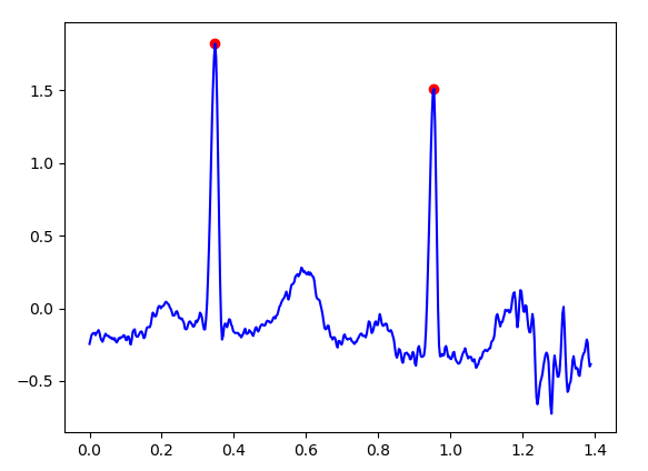
< Find all the peaks on ECG >
|
import numpy as np
import matplotlib.pyplot as plt
import scipy as sp
from scipy.misc import electrocardiogram
from scipy.signal import find_peaks
fs = 360;
x = electrocardiogram()[0:500];
t = (np.linspace(0,x.size,x.size) / fs)[0:500];
peaks,_ = find_peaks(x);
plt.plot(t, x,'b-');
plt.scatter(t[peaks],x[peaks],c='red');
plt.show();
|
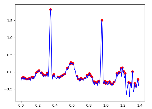
< Find the peaks above a threshold on ECG >
|
import numpy as np
import matplotlib.pyplot as plt
import scipy as sp
from scipy.misc import electrocardiogram
from scipy.signal import find_peaks
fs = 360;
x = electrocardiogram()[0:500];
t = (np.linspace(0,x.size,x.size) / fs)[0:500];
peaks,_ = find_peaks(x);
plt.plot(t, x,'b-');
plt.scatter(t[peaks],x[peaks],c='red');
plt.show();
|
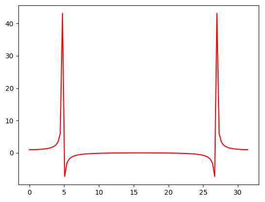
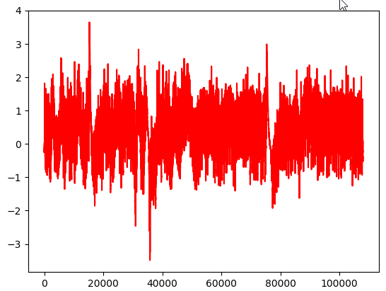
ECG (ElectroCardiogram)
|
import numpy as np
import matplotlib.pyplot as plt
import scipy as sp
import scipy.misc as spm
x = spm.electrocardiogram();
plt.plot(x,'r-');
plt.show();
|
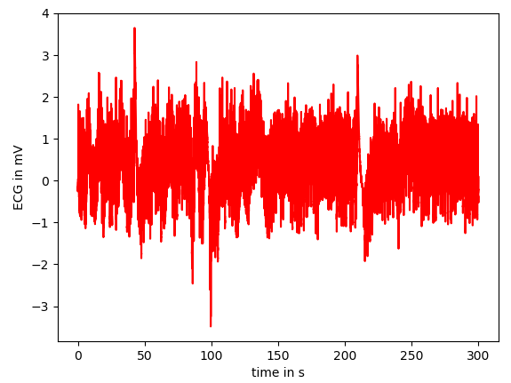
|
import numpy as np
import matplotlib.pyplot as plt
import scipy as sp
import scipy.misc as spm
fs = 360;
x = spm.electrocardiogram();
t = np.linspace(0,x.size,x.size) / fs;
plt.plot(t, x,'r-');
plt.xlabel('time in s');
plt.ylabel('ECG in mV');
plt.show();
|
|
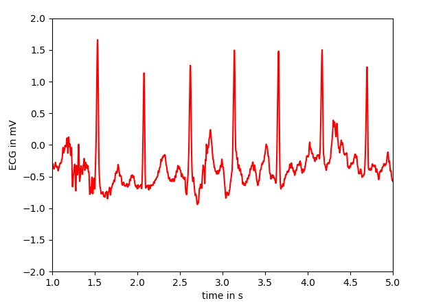
import numpy as np
import matplotlib.pyplot as plt
import scipy as sp
import scipy.misc as spm
fs = 360;
x = spm.electrocardiogram();
t = np.linspace(0,x.size,x.size) / fs;
plt.plot(t, x,'r-');
plt.xlim(1.0,5.0);
plt.ylim(-2,2);
plt.xlabel('time in s');
plt.ylabel('ECG in mV');
plt.show();
|
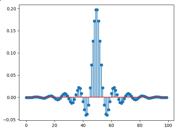
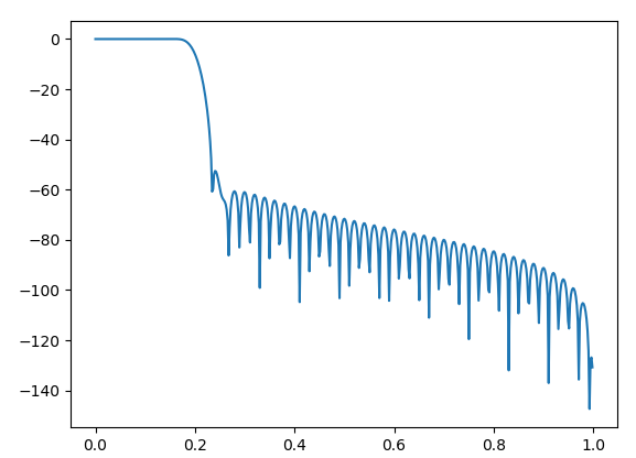
Low Pass Filter
|
import numpy as np
import matplotlib.pyplot as plt
import scipy as sp
from scipy import signal
n = 100;
b = signal.firwin(n,cutoff = 0.2, window = "hamming");
plt.stem(b);
plt.show();
|
|
import numpy as np
import matplotlib.pyplot as plt
import scipy as sp
from scipy import signal
n = 100;
a = 1;
b = signal.firwin(n,cutoff = 0.2, window = "hamming");
w,h = signal.freqz(b,a);
h_dB = 20 * np.log10(abs(h))
plt.plot(w/np.pi,h_dB);
plt.show();
|
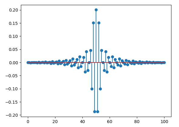
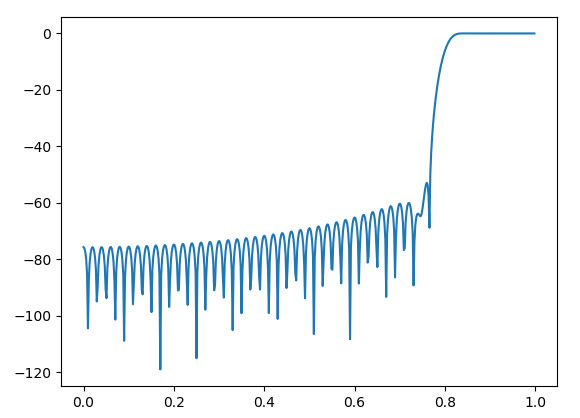
High Pass Filter
|
import numpy as np
import matplotlib.pyplot as plt
import scipy as sp
from scipy import signal
n = 101;
b = signal.firwin(n,cutoff = 0.8, window = "hamming",pass_zero = False);
plt.stem(b,use_line_collection = True);
plt.show();
|
|
import numpy as np
import matplotlib.pyplot as plt
import scipy as sp
from scipy import signal
n = 101;
a = 1;
b = signal.firwin(n,cutoff = 0.8, window = "hamming",pass_zero = False);
w,h = signal.freqz(b,a);
h_dB = 20 * np.log10(abs(h))
plt.plot(w/np.pi,h_dB);
plt.show();
|
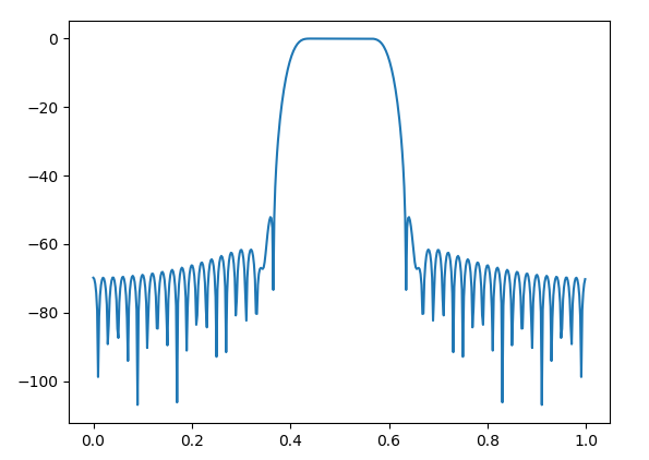
Band Pass Filter
|
import numpy as np
import matplotlib.pyplot as plt
import scipy as sp
from scipy import signal
n = 101;
b = signal.firwin(n,cutoff = [0.4,0.6], window = "hamming",pass_zero = False);
plt.stem(b,use_line_collection = True);
plt.show();
|
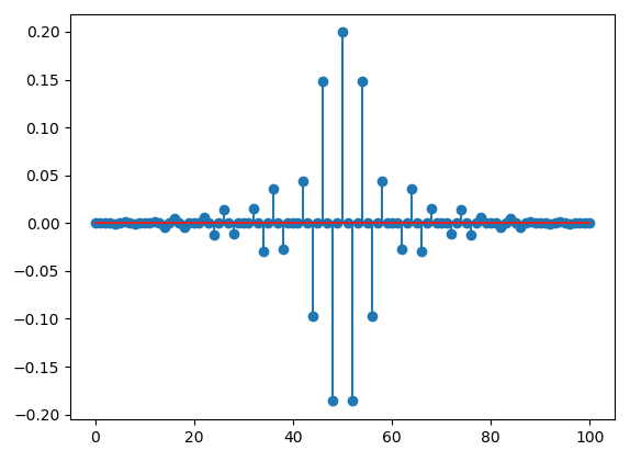
|
import numpy as np
import matplotlib.pyplot as plt
import scipy as sp
from scipy import signal
n = 101;
a = 1;
b = signal.firwin(n,cutoff = [0.4,0.6], window = "hamming",pass_zero = False);
w,h = signal.freqz(b,a);
h_dB = 20 * np.log10(abs(h))
plt.plot(w/np.pi,h_dB);
plt.show();
|
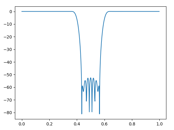
Band Stop Filter
|
import numpy as np
import matplotlib.pyplot as plt
import scipy as sp
from scipy import signal
n = 101;
b = signal.firwin(n,cutoff = [0.4,0.6], window = "hamming");
plt.stem(b,use_line_collection = True);
plt.show();
|
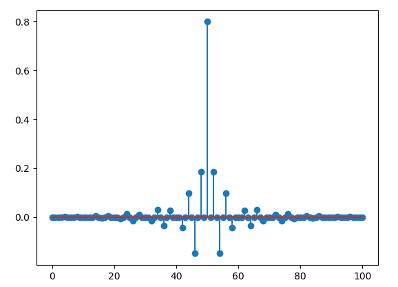
|
import numpy as np
import matplotlib.pyplot as plt
import scipy as sp
from scipy import signal
n = 101;
a = 1;
b = signal.firwin(n,cutoff = [0.4,0.6], window = "hamming");
w,h = signal.freqz(b,a);
h_dB = 20 * np.log10(abs(h))
plt.plot(w/np.pi,h_dB);
plt.show();
|
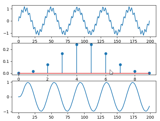
Applying Filter to Signal
|
import numpy as np
import matplotlib.pyplot as plt
import scipy as sp
from scipy import signal
t = np.linspace(0,10*np.pi,200);
sig = np.sin(t) + 0.2 * np.sin(10*t);
n = 10;
filter_taps = signal.firwin(n,cutoff = 0.2, window = "hamming");
sig_filtered = signal.lfilter(filter_taps, 1.0, sig)
plt.subplot(3,1,1);
plt.plot(sig);
plt.subplot(3,1,2);
plt.stem(filter_taps,use_line_collection = True);
plt.subplot(3,1,3);
plt.plot(sig_filtered);
plt.show();
|
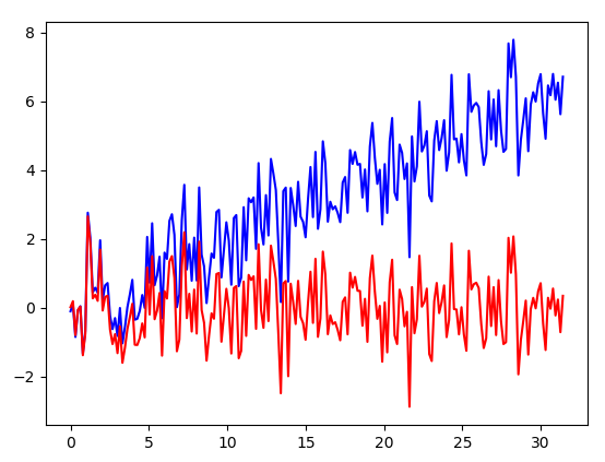
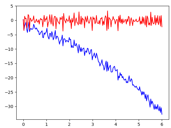
Detrending
< Detrending with detrend() >
|
import numpy as np
import matplotlib.pyplot as plt
import scipy as sp
from scipy import signal
t = np.linspace(0,10*np.pi,200);
x = 0.2*t + np.random.normal(size=len(t));
x_detrended = signal.detrend(x);
plt.plot(t, x,'b-');
plt.plot(t, x_detrended,'r-');
plt.show();
|
|
import numpy as np
import matplotlib.pyplot as plt
import scipy as sp
from scipy import signal
t = np.linspace(0,10*np.pi,200);
x = -0.5*pow(t + 2,2) + np.random.normal(size=len(t));
x_detrended = signal.detrend(x);
plt.plot(t, x,'b-');
plt.plot(t, x_detrended,'r-');
plt.show();
|
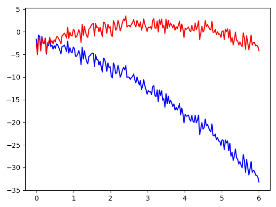
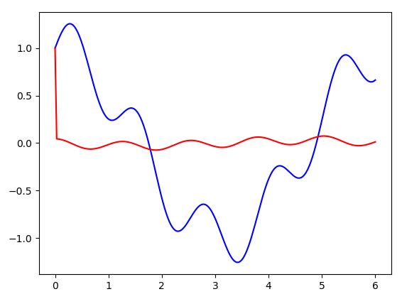
< Detrending with convolution() >
|
import numpy as np
import matplotlib.pyplot as plt
import scipy as sp
from scipy import signal
x = -0.5*pow(t + 2,2) + np.random.normal(size=len(t));
w = [1,-1];
x_detrended = np.convolve(x,w,mode='same');
plt.plot(t, x,'b-');
plt.plot(t, x_detrended,'r-');
plt.show();
|
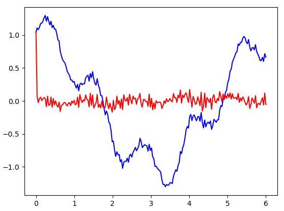
|
import numpy as np
import matplotlib.pyplot as plt
import scipy as sp
from scipy import signal
x = np.cos(t) + 0.3*np.sin(5*t);
w = [1,-1];
x_detrended = np.convolve(x,w,mode='same');
plt.plot(t, x,'b-');
plt.plot(t, x_detrended,'r-');
plt.show();
|
|
import numpy as np
import matplotlib.pyplot as plt
import scipy as sp
from scipy import signal
x = np.cos(t) + 0.3*np.sin(5*t);
x += 0.05*np.random.normal(size=len(t));
w = [1,-1];
x_detrended = np.convolve(x,w,mode='same');
plt.plot(t, x,'b-');
plt.plot(t, x_detrended,'r-');
plt.show();
|
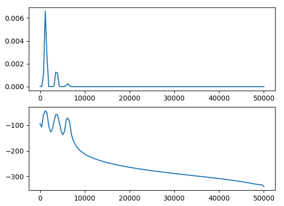
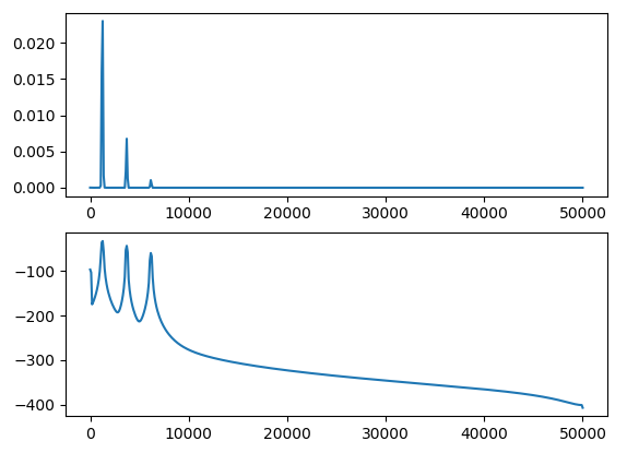
Welch
|
import numpy as np
import matplotlib.pyplot as plt
from scipy import signal, fft
N = 1000000;
fs = 100000;
dt = 1.0/fs;
fc = 1234.0;
amp = 2*np.sqrt(2);
t = dt * np.arange(N);
sig = np.cos(2*np.pi*fc*t) + 0.5*np.cos(3*2*np.pi*fc*t) + 0.2*np.cos(5*2*np.pi*fc*t);
sig = amp * sig;
freq,Pd = signal.welch(sig,fs);
plt.subplot(2,1,1);
plt.plot(freq,Pd);
plt.subplot(2,1,2);
plt.plot(freq,20*np.log10(Pd));
plt.show();
|
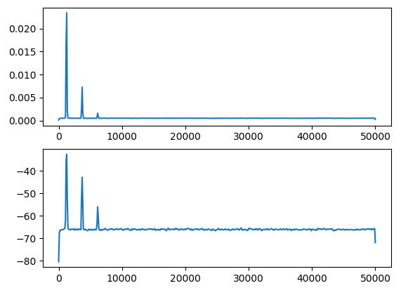
|
import numpy as np
import matplotlib.pyplot as plt
from scipy import signal, fft
N = 1000000;
fs = 100000;
dt = 1.0/fs;
fc = 1234.0;
amp = 2*np.sqrt(2);
t = dt * np.arange(N);
sig = np.cos(2*np.pi*fc*t) + 0.5*np.cos(3*2*np.pi*fc*t) + 0.2*np.cos(5*2*np.pi*fc*t);
sig = amp * sig;
freq,Pd = signal.welch(sig,fs,nperseg=1024); # change resolution with nperseg option
plt.subplot(2,1,1);
plt.plot(freq,Pd);
plt.subplot(2,1,2);
plt.plot(freq,20*np.log10(Pd));
plt.show();
|
|
import numpy as np
import matplotlib.pyplot as plt
from scipy import signal, fft
N = 1000000;
fs = 100000;
dt = 1.0/fs;
fc = 1234.0;
amp = 2*np.sqrt(2);
n_amp = 0.0001 * fs/2;
t = dt * np.arange(N);
sig = np.cos(2*np.pi*fc*t) + 0.5*np.cos(3*2*np.pi*fc*t) + 0.2*np.cos(5*2*np.pi*fc*t);
sig = amp * sig;
sig = sig + np.random.normal(scale=n_amp, size=t.shape); # add noise for noise floor
freq,Pd = signal.welch(sig,fs,nperseg=1024); # change resolution with nperseg option
plt.subplot(2,1,1);
plt.plot(freq,Pd);
plt.subplot(2,1,2);
plt.plot(freq,20*np.log10(Pd));
plt.show();
|
Reference :
[1]
|
|