Quantum Computing
Deutsch Algorithm
Deutsch came up with this algorithm in 1985 that was a big deal in quantum computing. It showed how a quantum algorithm could solve a certain problem way faster than classical algorithms.
The goal was to compare what quantum vs classical computers could do efficiently. Scientists thought quantum would be faster, but didn't have examples yet. Deutch algorithm is a kind of first quantum algorithm that shows the case where quantum algorithm can work way faster than classical algorithm.
This algorithm is based on a simple situation / question illustrated below.
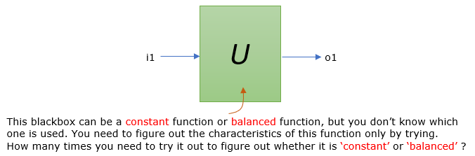
Here the definition of 'constant' and 'balance' function can be represented in truth tables as follows.
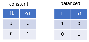
Constant Function : Whatever the input value is, output value is always same ('1' in this example)
Balanced Function : Output value is always different from the input value whatever it is
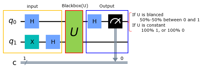
What Deutch algorithm shows is :
- In classical algorithm, you need to run twice to figure out whether the blackbox is 'constant' or 'balanced'
- In quantum algorithm, you can figure it out with only one trial
The implementation of Deutch algorithm is as follows :
Qiskit Example
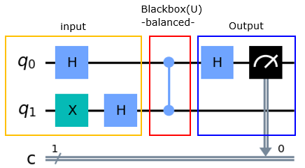
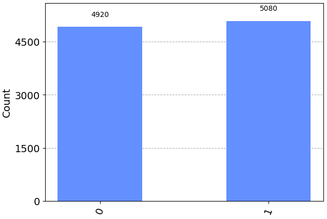
Example 01 > Balanced Function
|
from qiskit import QuantumCircuit, execute, Aer, ClassicalRegister, QuantumRegister from qiskit.visualization import plot_histogram
# Quantum and classical registers qreg_q = QuantumRegister(2, 'q') creg_c = ClassicalRegister(1, 'c')
# Create quantum circuit circuit = QuantumCircuit(qreg_q, creg_c)
# Put qubit 0 into superposition circuit.h(qreg_q[0])
# Put qubit 1 into superposition circuit.x(qreg_q[1]) circuit.h(qreg_q[1])
# Entangle qubits with CZ gate (balanced oracle) circuit.cz(qreg_q[0], qreg_q[1])
# Apply final H gate circuit.h(qreg_q[0])
# Measurement circuit.measure(qreg_q[0], creg_c[0]) |
|
|
|
# Simulate the circuit simulator = Aer.get_backend('qasm_simulator') job = execute(circuit, simulator, shots=10000) result = job.result()
# Get counts and plot the histogram counts = result.get_counts(circuit) plot_histogram(counts) |
|
|
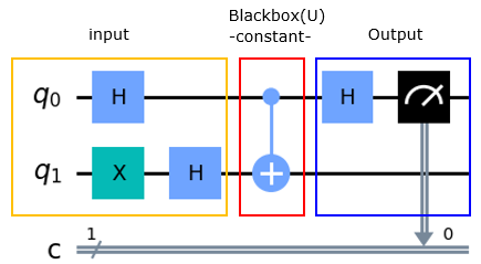
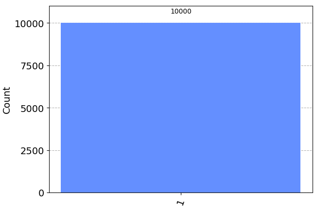
Example 02 > Constant Function
|
from qiskit import QuantumCircuit, execute, Aer, ClassicalRegister, QuantumRegister from qiskit.visualization import plot_histogram
# Quantum and classical registers qreg_q = QuantumRegister(2, 'q') creg_c = ClassicalRegister(1, 'c')
# Create quantum circuit circuit = QuantumCircuit(qreg_q, creg_c)
# Put qubit 0 into superposition circuit.h(qreg_q[0])
# Put qubit 1 into superposition circuit.x(qreg_q[1]) circuit.h(qreg_q[1])
# Entangle qubits with CX(CNOT) gate (balanced oracle) circuit.cx(qreg_q[0], qreg_q[1])
# Apply final H gate circuit.h(qreg_q[0])
# Measurement circuit.measure(qreg_q[0], creg_c[0])
# Draw the circuit. circuit.draw('mpl') |
|
|
|
# Simulate the circuit simulator = Aer.get_backend('qasm_simulator') job = execute(circuit, simulator, shots=10000) result = job.result()
# Get counts and plot the histogram counts = result.get_counts(circuit) plot_histogram(counts) |
|
|
Reference