Quantum Computing
Shor's Algorithm
Shor's Algorithm is a quantum computing algorithm designed for efficiently factoring large numbers, a task that is computationally very difficult for classical computers. It was developed by mathematician Peter Shor in 1994 and is famous for its ability to break commonly used cryptographic protocols like RSA. The algorithm works by exploiting the principles of quantum superposition and entanglement to perform calculations at an exponentially faster rate than classical algorithms. This efficiency arises from its quantum Fourier transform component, which processes multiple potential factors simultaneously, vastly outperforming traditional factoring methods on sufficiently large numbers when run on a quantum computer.
Shor's takes an integer N to be factored and an integer a coprime to N. The algorithm finds the period r of the function f(x) = a^x mod N using a quantum period-finding subroutine. Once r is found, N can be factored efficiently on a classical computer by calculating gcd(a^(r/2) ± 1, N).
The key insight is that a quantum computer can efficiently find the period r, whereas the best known classical algorithms have exponential runtime. Factoring large integers is believed to be classically hard but by using properties of quantum superposition and interference, Shor's algorithm can do it polynomial time - an exponential speedup over the best classical algorithms. This demonstrates the power quantum algorithms have over classical for certain problems.
Overall descriptions of the implementation of Shor's algorithm can be described as follows :
1.Quantum Register Preparation
- Initialize two quantum registers - one to store the input and periodic state, another to store the measured output.
- Create uniform superposition in the input register through Hadamard gates.
- Variation: Alternative initializations may be used depending on the quantum hardware limitations or to optimize the algorithm's efficiency.
2. Modular Exponentiation Circuit
- This creates the states |x>|a^x mod N> through a sequence of modular multiplication and exponentiation gates controlled by the input register.
- Variation: The implementation of modular exponentiation can vary, including more efficient quantum arithmetic to reduce gate counts and adapt to hardware constraints.
3. Quantum Fourier Transform
- Apply QFT to the input register. This creates a state where probabilities of measuring x values are peaked at multiples of the period r.
- Variation: Some implementations might use an approximate QFT to simplify the circuit, especially in near-term quantum devices with limited qubits.
4. Measurement
- Measure the state of the input register. Get a set of sampled x values.
- Variation: Measurement strategies might differ, especially to minimize errors and maximize the information gained about the period r.
5. Classical Post-Processing
- Apply mathematical techniques like continued fractions on the set of x values to determine the period r.
- Variation: Different classical algorithms for extracting the period r from the measurements can be used, depending on computational efficiency and accuracy.
- With r, use Euclid's algorithm to factor N efficiently.
- Variation: The choice of algorithm for finding the factors, once r is known, may vary, including more sophisticated methods for handling special cases.
NOTE : Is there any formal relation between the size of N (the number to be factored) and number of required Qbit ?
Yes, there is a formal relation between the size of the integer N to be factored and the number of qubits required in Shor's algorithm
In general, the number of qubits scales linearly with the bit size of the integer being factored. Larger n requires exponentially more classical computational power, but only a linear increase in quantum resources. This polynomial vs exponential scaling is why Shor's provides an enormous speedup.
The number of qubits required depends on the size of N measured in bits. If N is an n-bit integer, then the number of qubits Q needed is:
Q = 2n + 3
Here is the breakdown:
- n qubits are needed to store the input number N using a quantum register
- n qubits are needed for the periodic quantum state register
- 2 qubits are needed for the modular exponentiation circuit
- 1 qubit is needed for an ancilla/work space
- So total is 2n qubits for the two registers + 3 extra qubits = 2n + 3 qubits.
For example, factoring a 32-bit integer would require:
n = 32 (the integer size) ==> N = 4,294,967,295 (a common 32-bit unsigned integer maximum value)
Therefore, Q = 2*32 + 3 = 67 qubits
Another example for n=2048 (most widely used RSA key size)
n = 2048 (RSA key size)
Q = 2*2048 + 3 Q = 4096 + 3 Q = 4099
Qiskit Code
|
pip install qiskit_algorithms |
Build Quantum Circuit and Run
|
from qiskit import QuantumCircuit, Aer, execute from qiskit.visualization import plot_histogram from math import pi import matplotlib.pyplot as plt
def apply_cphase(qc, control_qubit, target_qubit, theta): # Apply Controlled-Phase gate qc.cp(theta, control_qubit, target_qubit)
def apply_qft(circuit, n): """Applies the QFT on the first n qubits in circuit""" for qubit in range(n): # Apply the Hadamard gate circuit.h(qubit) # Apply the controlled phase gates for control_qubit in range(qubit): theta = pi / (2 ** (qubit - control_qubit)) apply_cphase(circuit, control_qubit, qubit, theta)
# Apply SWAP gates to reverse the order of the qubits for qubit in range(n // 2): circuit.swap(qubit, n - qubit - 1)
# Define the number of qubits n_qubits = 4
# Initialize the quantum circuit qc = QuantumCircuit(n_qubits, n_qubits)
# Apply QFT to the quantum circuit apply_qft(qc, n_qubits)
# Measure the qubits for qubit in range(n_qubits): qc.measure(qubit, qubit)
# Draw the circuit #qc.draw(output='mpl') #plt.show()
# Execute the circuit on a simulator backend = Aer.get_backend('qasm_simulator') result = execute(qc, backend, shots=1024*4).result() counts = result.get_counts(qc)
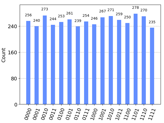
# Display the results print(counts) plot_histogram(counts) |
|
{'1011': 259, '0001': 240, '1100': 250, '1000': 246, '0110': 239, '1101': 278, '0011': 244, '0111': 254, '1110': 270, '1001': 267, '0101': 261, '0000': 256, '0010': 273, '1111': 235, '1010': 271, '0100': 253}
|
Draw the Circuit
|
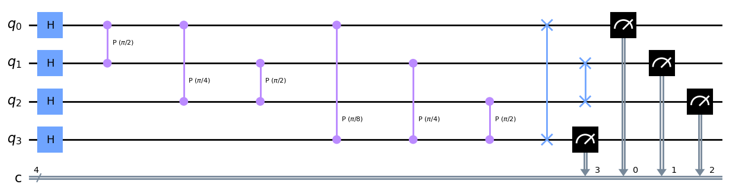
qc.draw('mpl') |
|
|
Classical Post Processing
|
from math import gcd from fractions import Fraction from random import randint
# Define the number you want to factor N = 15
# Choose a random number 'a' that is coprime to N # It's a good idea to check if a is actually coprime to N a = randint(2, N-1) while gcd(a, N) != 1: a = randint(2, N-1) # Choose a new 'a' if necessary
# Define 'counts' as the output from the quantum circuit's measurements # Replace this with your actual counts from the Qiskit simulation counts = { '0000': 100, '0001': 50, '0010': 75, # ... (rest of your counts) }
# Define the number of qubits used in the QFT n_qubits = 4
# Define Q as 2 to the power of the number of qubits used in the QFT Q = 2**n_qubits
# Find the period r using the continued fraction expansion potential_rs = set() for measured_value in counts: measured_value_int = int(measured_value, 2) for denominator in range(2, Q): fraction = Fraction(measured_value_int, Q).limit_denominator(denominator) if fraction.denominator not in potential_rs and abs(fraction - Fraction(measured_value_int, Q)) < 1/Q: potential_rs.add(fraction.denominator)
# Attempt to find factors for each potential r factors = set() for r in potential_rs: if r % 2 == 0 and a**(r//2) % N != N - 1: # additional check to ensure a^(r/2) is not congruent to -1 mod N possible_factor_1 = gcd(a**(r//2) - 1, N) possible_factor_2 = gcd(a**(r//2) + 1, N) if 1 < possible_factor_1 < N: factors.add(possible_factor_1) if 1 < possible_factor_2 < N: factors.add(possible_factor_2)
# Output the non-trivial factors if factors: print(f"The non-trivial factors of {N} are: {factors}") else: print(f"No non-trivial factors found. The period might not be correct or 'a' might not be a good choice.") |
|
The non-trivial factors of 15 are: {3, 5} |
Details of the Circuit
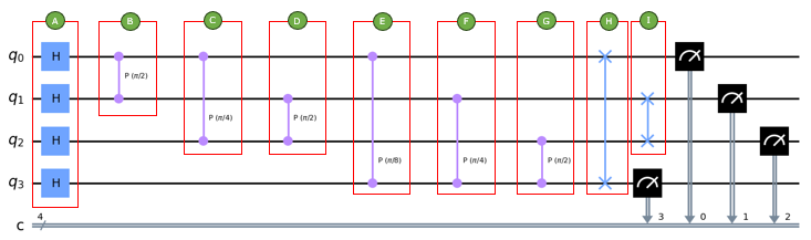
This is to implement the Quantum Fourier Transform (QFT) on a 4-qubit register. The QFT is used in quantum algorithms, most famously in Shor's algorithm for integer factorization, to transform the quantum state into one where the periodicity of a function is evident. The periodicity can then be extracted from the measurement outcomes and used to find factors of integers or solve other problems related to periodicity.
If this circuit is meant to be a part of Shor's algorithm, the presence of additional Hadamard gates in Block G is unusual and may be specific to the particular variant or adaptation of the QFT or the algorithm. If it's not delivering the expected results, the modifications in Block G would be the first thing to review.
The circuit is broken down into several labeled blocks:
- Block A (Hadamard Gates):
- Each qubit (q0, q1, q2, q3) is passed through a Hadamard gate. The Hadamard gate puts each qubit into a superposition of |0> and |1>. If the initial state of each qubit was |0>, the state after this block would be an equal superposition of all the basis states of the 4-qubit register.
- Block B (Controlled Phase Rotation Gate):
- This gate is a controlled phase rotation gate, specifically a controlled-R(pi/2) rotation, which is sometimes denoted as cR(pi/2).
- The gate applies a phase shift of pi/2 (90 degrees) to the target qubit(q1), but only when the control qubit(q0) is in the state |1>.
- If the control qubit is in the state |0>, then there is no phase shift applied to the target qubit.
- This operation creates phase relationships between the qubits, which is a crucial step in the Quantum Fourier Transform (QFT).
- Block C (Controlled Phase Rotation Gate):
- This gate is a controlled phase rotation gate, specifically a controlled-R(pi/2) rotation, which is sometimes denoted as cR(pi/2).
- The gate applies a phase shift of π/4 (45 degrees) to the target qubit(q2), but only when the control qubit(q0) is in the state |1>.
- If the control qubit is in the state |0>, then there is no phase shift applied to the target qubit.
- This operation creates phase relationships between the qubits, which is a crucial step in the Quantum Fourier Transform (QFT).
- Block D (Controlled Phase Rotation Gate):
- This gate is a controlled phase rotation gate, specifically a controlled-R(pi/2) rotation, which is sometimes denoted as cR(pi/2).
- The gate applies a phase shift of pi/2 (90 degrees) to the target qubit(q2), but only when the control qubit(q1) is in the state |1>.
- If the control qubit is in the state |0>, then there is no phase shift applied to the target qubit.
- This operation creates phase relationships between the qubits, which is a crucial step in the Quantum Fourier Transform (QFT).
- Block E (Controlled Phase Rotation Gate):
- This gate is a controlled phase rotation gate, specifically a controlled-R(pi/2) rotation, which is sometimes denoted as cR(pi/2).
- The gate applies a phase shift of π/8 (22.5 degrees) to the target qubit(q8), but only when the control qubit(q0) is in the state |1>.
- If the control qubit is in the state |0>, then there is no phase shift applied to the target qubit.
- This operation creates phase relationships between the qubits, which is a crucial step in the Quantum Fourier Transform (QFT).
- Block F (Controlled Phase Rotation Gate):
- This gate is a controlled phase rotation gate, specifically a controlled-R(pi/2) rotation, which is sometimes denoted as cR(pi/2).
- The gate applies a phase shift of π/4 (45 degrees) to the target qubit(q3), but only when the control qubit(q1) is in the state |1>.
- If the control qubit is in the state |0>, then there is no phase shift applied to the target qubit.
- This operation creates phase relationships between the qubits, which is a crucial step in the Quantum Fourier Transform (QFT).
- Block G (Controlled Phase Rotation Gate):
- This gate is a controlled phase rotation gate, specifically a controlled-R(pi/2) rotation, which is sometimes denoted as cR(pi/2).
- The gate applies a phase shift of pi/2 (90 degrees) to the target qubit(q3), but only when the control qubit(q2) is in the state |1>.
- If the control qubit is in the state |0>, then there is no phase shift applied to the target qubit.
- This operation creates phase relationships between the qubits, which is a crucial step in the Quantum Fourier Transform (QFT).
- Block H (SWAP Gate):
- This SWAP gate is used to exchange the quantum states of two qubits. After applying a SWAP gate, the state of the first qubit(q0) becomes the state of the second qubit(q3) and vice versa. This is particularly useful in quantum algorithms where the position of qubits relative to each other is significant, such as in the Quantum Fourier Transform, where the order of qubits is reversed as the last step.
- Block G (SWAP Gate):
- This SWAP gate is used to exchange the quantum states of two qubits. After applying a SWAP gate, the state of the first qubit(q1) becomes the state of the second qubit(q2) and vice versa. This is particularly useful in quantum algorithms where the position of qubits relative to each other is significant, such as in the Quantum Fourier Transform, where the order of qubits is reversed as the last step.
Reference