I think one of the most widely adopted application of AI/ML in physical layer is for CSI report process. In this note, I am trying to consollidate various concepts and ideas from different sources.

• Comparison of Non-AI and AI-enabled CSI Feedback Frameworks
• Use Case and Models
• Report Enhancement
• Report Prediction
• TDoc Snapshots
• R1-2400046: Discussion on AIML for CSI prediction
• R1-2400047: Discussion on AIML for CSI prediction
• R1-2400094: Discussion on other aspects of AI/ML model and data on AI/ML for NR air-interface
• R1-2400095: Discussion on potential performance enhancements/overhead reduction with AI/ML-based CSI feedback compression
• R1-2400146: Discussion on CSI prediction for AI/ML
• R1-2400150: Discussion on CSI compression for AI/ML
• R1-2500051 : Discussion of CSI compression on AI/ML for NR air interface
• Reference
• 3GPP TR/TS/General
• 3GPP TDocs
• General Reading

Comparison of Non-AI and AI-enabled CSI Feedback Frameworks

NOTE :  The term 'sparsity' in this context mean that the CSI can be represented in a sparse or compressed form in a certain domain, such as the angular or delay domain. This sparsity allows for more efficient transmission of CSI from the user equipment (UE) to the base station (BS), as the sparse representation can be transmitted with less data than the full CSI.

As an example, let's consider a wireless communication system where a base station (BS) communicates with multiple user equipment (UE) devices in a multi-path environment. In such a scenario, the Channel State Information (CSI) can be represented as a matrix, where each entry represents the channel gain from a specific transmit antenna at the BS to a receive antenna at a UE over a specific path.

In a typical urban environment, there are only a limited number of paths (due to buildings, trees, etc.) that the signal can take from the BS to a UE. This means that most of the paths do not exist, and therefore, the corresponding entries in the CSI matrix are zero. This results in a sparse matrix, i.e., a matrix with mostly zero entries.

This is the sparsity in the context of CSI feedback. By exploiting this sparsity, advanced signal processing techniques such as compressive sensing can be used to compress the CSI matrix for feedback from the UE to the BS, reducing the amount of data that needs to be transmitted and therefore saving bandwidth.

Use Case and Models

There can be various type of AI/ML models applicable to this application and I will try to collect those models from various source.

Report Enhancement

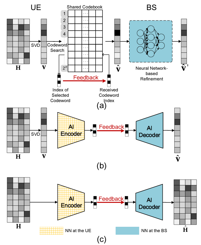
Let me start with models described in the paper AI for CSI Feedback Enhancement in 5G-Advanced. The frameworks proposed in this paper is well summarized by the following figure.

Source : AI for CSI Feedback Enhancement in 5G-Advanced

These model can be summarized and compared as in a table as follows.

NOTE :What does it mean by 'Implicit' and 'Explicit' ?

• Implicit CSI Feedback: In this case, the UE does not send the full CSI back to the BS. Instead, it sends a more compact representation, such as a precoding matrix or a codeword index from a predefined codebook. The BS then uses this information to infer the CSI. This method reduces the amount of data that needs to be sent back to the BS, saving bandwidth. However, it may not be as accurate as explicit feedback, especially in rapidly changing or complex environments.
• Explicit CSI Feedback: In this case, the UE sends the full CSI back to the BS. This method can provide more accurate and detailed information about the channel to the BS, which can be beneficial for optimizing communication. However, it requires more bandwidth to send the full CSI, and it may also require more complex processing at the UE and the BS.

I found another well described method from Mathworks document : CSI Feedback with Autoencoders. I think the best part of this documents is to show the detailed procedure of each steps along the entire process.

Overall process is illustrated as follows : As you see here, the entire channel coefficient for every resource elements of every antenna is preprocessed (data reduction) and encoded (compressed), and sent to reciever and recovered to channel coefficient for every subcarriers and antenna.

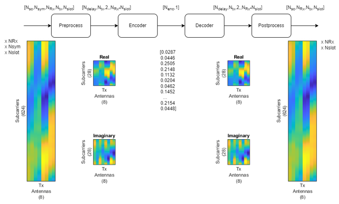
High leve descriptions of this process is as follows :

• Preprocess:
• The input data, which has dimensions [N_sc, N_sym, N_rx, N_tx, N_slot], represents the CSI matrix, where N_sc is the number of subcarriers, N_sym is the number of symbols, N_rx is the number of receiver antennas, N_tx is the number of transmitter antennas, and N_slot is the number of time slots.
• The preprocessing stage likely includes operations such as normalization, noise reduction, and possibly feature extraction, to prepare the CSI data for the encoding stage. The heatmap suggests a distribution of signal characteristics across subcarriers and transmitter antennas before this preprocessing.
• Encoder:
• This stage compresses the preprocessed CSI data into a lower-dimensional space. The encoder is part of the autoencoder architecture and is designed to capture the most important features of the input data.
• The output of the encoder is a compact representation, often referred to as a "code" or "latent space representation". The numbers shown in the brackets ([0.0287, 0.0446, ...]) represent this compressed feature vector, which significantly reduces the dimensionality from the original input (a few numbers compared to potentially thousands in the input data).
• Decoder:
• The decoder is the second part of the autoencoder that attempts to reconstruct the original data from the compressed form created by the encoder. The objective is to have the output of the decoder match the original input data as closely as possible.
• This step is critical for understanding how well the autoencoder can compress and reconstruct the CSI information, which is essential for reducing the overhead in feedback channels.
• Postprocess:
• After the decoder, there might be some postprocessing operations. These could include reshaping the data back to its original dimensions, scaling it back to its original range if normalization was applied, or applying some form of error correction.
• The final heatmap on the right of the diagram looks similar to the initial input heatmap, which implies that the autoencoder is able to reconstruct the CSI data effectively from the compressed representation.

Out of the entire process, Preprocessing step can be broken down into followint steps. I think a good thing of the matlap document explains about this preprocessing step whereas most of the academic papers explain only about the core part (encoder/decoder part).

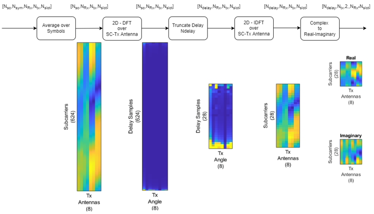
High level description for each step is as follows :

• Average over Symbols:
• The CSI is initially represented as a multidimensional matrix with dimensions corresponding to the number of subcarriers, symbols, receiver antennas, transmitter antennas, and time slots.
• The first step is to average the signal over multiple symbols to stabilize the CSI estimate by reducing noise and transient effects. This averaging process helps in obtaining a more reliable representation of the channel characteristics.
• 2D - DFT over SC-Tx Antenna:
• A two-dimensional Discrete Fourier Transform (2D-DFT) is applied over the subcarriers and transmitter antennas.
• The DFT over the transmitter antennas reveals the spatial frequency components that correspond to different angles of departure (AoD) for the transmitted signal. Essentially, this can provide the steering vectors for beamforming.
• The DFT over the subcarriers helps understand how the channel response varies across different frequencies.
• Note that x axis and y xis after this step becomes angle and delay samples.
• Truncate Delay Ndelay
• After the 2D-DFT, the signal in the delay domain is truncated to retain only the first Ndelay samples.
• This truncation step is a form of dimensionality reduction, keeping the most significant delay paths which represent the channel's impulse response.
• 2D - IDFT over SC-Tx Antenna:
• A two-dimensional Inverse Discrete Fourier Transform (2D-IDFT) is then applied to the truncated signal.
• This step is the reverse of the 2D-DFT and transforms the signal back into the spatial and subcarrier domains. It's essentially reconstructing the signal from its spatial frequency components.
• Complex to Real-Imaginary:
• The complex-valued matrix resulting from the 2D-IDFT is then separated into its real and imaginary parts.
• This separation is necessary because in many practical systems, especially those that involve hardware processing, it's easier to deal with real and imaginary parts separately.

As in any type of machine learning algorithm, it is crucial and challenging to figure out how to train the model. It is even more challenging in case of auto encoder model because one model is seprated into different location : half of the model (encoder) is located in UE and half of the model is located in RAN. The challenges and possible workaround is well summarized in An Overview of the 3GPP Study on Artificial Intelligence for 5G New Radio as illustrated below.

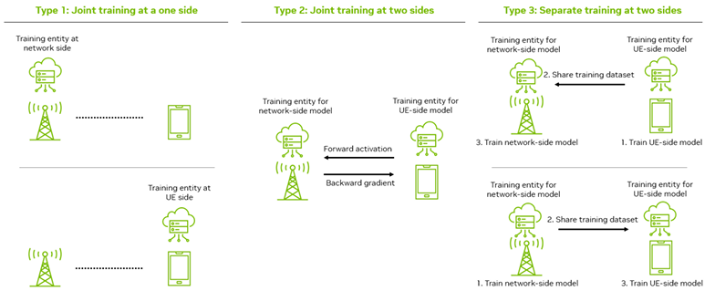
Image Source : An Overview of the 3GPP Study on Artificial Intelligence for 5G New Radio

This is overall description of the training method shown in this illustration.

• Type 1: Joint training at one side - Training is conducted solely at one entity, either at the network side or the user equipment (UE) side.
• Type 2: Joint training at two sides - Training involves both the network and UE sides. The network-side model sends forward activation to the UE-side model, which then sends back the backward gradient. It means the training process is collaborative. The network model performs part of the computation and sends the result to the UE model, which continues the computation and sends back the necessary adjustments (gradients) to the network model. 'Forward activation' and 'Backward gradient' refer to the components of the backpropagation algorithm used in training neural networks. In joint training, these processes are distributed between the network and user equipment, allowing for a collaborative model training that takes advantage of computational resources and data available on both sides. Here's a simplified breakdown:
• Forward Activation: This is the process where input data is passed through the network layer by layer until the output layer is reached. At each layer, the input is transformed using weights and a non-linear activation function. The final output is the 'activation' that is then used to make predictions.
• Backward Gradient: After the forward pass, the output is compared to the desired outcome using a loss function, and the error is calculated. During the backward pass, this error is propagated back through the network, which involves computing the gradient of the loss function with respect to the weights of the network. This gradient is used to update the weights in the network to minimize the loss, hence the term 'backward gradient'.
• Type 3: Separate training at two sides - Both network and UE sides train their respective models separately but share a training dataset. The nature of the training dataset exchanged is usually in the form of feature sets or labeled data samples that are relevant to both the network-side and user equipment (UE)-side models. The exchange of such datasets aims to ensure that both models, though trained separately, benefit from a harmonized understanding of the environment they operate in, leading to improved overall performance when deployed in a real-world setting. The dataset would typically consist of:
• Data samples that have been preprocessed and labeled from both network and UE perspectives.
• Information that is relevant for both models to learn from, which might include signal characteristics, network conditions, user behavior, or other context-specific information that can improve the model's performance on both ends.

Report Prediction

Getting the accurate CSI report at the proper timing is crucial for physical layer operation of most of wireless system. It is especially true for the system like 5G/NR which uses high degree of MIMO technology. However, getting the CSI report all the time usually requires very frequent CSI report and the frequent CSI report causes huge overhead. For example, based on my observation. The most frequent CSI report interval that I see from live network of 5G/NR seems to be 40 ms, 80 ms, 160 ms. However, there can be so many things happening in radio channel over those period (e.g, 40 ms) and the CSI report that gNB just got would not be accurate enough to use for now or right near future as illustrated below.

In orther words, the motivation for using AI/ML algorithms for Channel State Information (CSI) prediction is to address the issue of channel aging, which is the delay between when CSI is reported and when it is used by the gNB (gNodeB). This delay leads to the reported CSI being outdated, particularly at higher UE (User Equipment) speeds. This is a significant issue in MU-MIMO (multi-user multiple-input multiple-output) scenarios, especially with massive MIMO deployments where the performance is negatively impacted by the movement of UEs at medium to high speeds. AI/ML-based CSI prediction aims to mitigate the effects of outdated CSI by forecasting future CSI states, enabling more accurate and timely adjustments to the wireless network, enhancing overall communication performance.

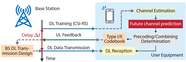
Image Source : Predicting Future CSI Feedback For Highly-Mobile Massive MIMO Systems

What would be the solution to increase the accuracy of CSI value over the whole period before next report ? The answer is to 'properly' estimate the CSI value for the periiod between the latest CSI report and the next coming report.

It is easy to say, but not easy at all to do. There can be various algorithms to predict a specific values from the past data even before AI/ML came out. It would be natural to trying to think of applying AI/ML for this application.

In conclusion, the dynamic nature of the wireless environment and the massive use of MIMO technology in 5G/NR systems present significant challenges in obtaining accurate and timely CSI reports. The high overhead associated with frequent CSI reporting only amplifies these difficulties. However, we can look towards intelligent solutions to address these challenges. AI and ML algorithms are promising tools that can "fill in the gaps" by predicting CSI values in between report intervals, thereby increasing the overall accuracy of the CSI report. While the implementation of such algorithms is not trivial, their potential to significantly enhance the efficiency and effectiveness of CSI reports cannot be overstated. It is an avenue worth exploring, offering us the potential to push the boundaries of our wireless systems to even greater heights. As we move forward, the integration of AI/ML into wireless communication systems should be a key focus in our pursuit of optimized performance and reliability.

What type of Deep Learning Model can be used for this type of application ?

Since the main focus of this application is to predict a certain value in time domain, the typical models for sequence prediction like RNN, LSTM, GRU would be the candidates that pops up in your head right away. But in some researches more conventional model like CNN is shown to work on this type of application.

Following is an example of applying CNN for CSI prediction. The frame proposed in this paper uses a 3-D convolutional neural network to capture temporal, spatial, and frequency correlations of downlink channel samples. The proposed model significantly improves performance compared to the sample-and-hold approach and mitigates the impact of the dynamic communication environment.

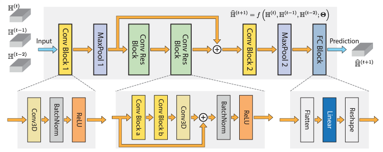
Image Source : Predicting Future CSI Feedback For Highly-Mobile Massive MIMO Systems

Overall description of the model (CNN model) proposed in this paper is as follows :

• Input: The input to the model is the past L channel observations.
• Conv Block 1 and Conv Block 2: These are convolutional blocks that include extra normalization layers and activation layers. They build on top of the 3-D convolutional layer.
• Conv Res Block: This is a convolutional residual block built on top of the convolutional block. It adopts a residual architecture, which is mainly used for extracting deeper features that are hardly found by shallow networks while keeping the training experience efficient.
• MaxPool 1 and MaxPool 2: These are max-pooling layers used to reduce the dimensionality of the input, which helps to reduce the number of parameters in the last fully connected layer.
• FC Block: This is a fully-connected block employed to reshape the output to have the desired dimension.
• Prediction: The output of the model is the predicted future channel state information.

NOTE : there is a stage where the output of MaxPool1 and the output of Conv Res Block. What is the purpose of it ?

The combination of the output of MaxPool1 and the Conv Res Block is a key part of the proposed deep learning model's architecture. This combination is a feature of the residual architecture used in the model.

The main purpose of introducing the second max-pooling layer (MaxPool2) is to reduce the number of parameters in the last fully connected layer (FC Block), as normally, Nt and K are relatively large.

• Nt refers to the number of antennas at the base station. It's a parameter that represents the transmit dimension in the spatial domain of the system.
• K refers to the number of resource blocks. It's a parameter that represents the frequency dimension of the system

The residual architecture is used to extract deeper features that are hardly found by shallow networks while keeping the training experience efficient. The output of the MaxPool1 and the Conv Res Block are combined and passed through another Conv Block (Conv Block 2) and then through MaxPool2. This process allows the model to capture more complex and abstract features from the input data, which can improve the accuracy of the model's predictions.

In short, this combination allows the network to learn from both the original features and the transformed features, which can help to improve the model's performance.

TDoc Snapshots

TDoc gives a lot of insights and intuitive explanations that are not usually provided by TS (Test Specification) but in many cases you may feel difficulties to catch up what a TDoc is talking about unless you tracked down the topics from the beginning. The discussions in TDocs proceed incrementaly and refer to many terms in previous TDocs without the detailed explanations. In order to catch up the document, I would suggest you to give careful readings on several TDocs released at the very early discussion and get familiar with core concepts and key terminologies. In this section, I want to note those core concepts and terminologies from TDoc based on my personal criteria.

R1-2400046: Discussion on AIML for CSI prediction

This is about CSI feedback enhancement [RAN1] with a few high level objectives as follows :

• CSI Compression (Two-sided Model):
• Balance performance with complexity and overhead.
• Consider broader compression methods:
• Spatial/temporal/frequency compression.
• Cell/site-specific models.
• Explore CSI compression combined with prediction.
• Aim for improvements over non-AI/ML approaches from Release 18.
• Tackle challenges in inter-vendor training collaboration.
• CSI Prediction (One-sided Model):
• Investigate performance improvements over Release 18's non-AI/ML methods.
• Evaluate the associated complexity.
• Examine the potential for cell/site-specific models.
• Aim for enhanced performance gains.

UE side model vs Network side model

As in other cases, we can think of two different model : UE side model and Network side model

UE side model

In this model, NW just instruct UE to perform the procedure for executing AI model and UE performs the procedure - Data Collection, Model Training and Model Inference.

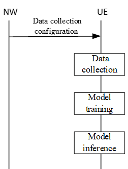
• Core Concept: UE measures reference signals, stores data, and trains machine learning models locally.
• Requirements:
  • Enhanced UE with computational power and storage space.
• Advantages:
  • Zero reporting overhead (with online training).
  • Potentially larger, richer datasets for training.
  • Can enhance privacy in some use cases.

NW side model

In this mode, Network request UE to collect and send the report for model training to Network and Network collect traininng data from UE report and perform model training. And then Network transfer the model to UE and UE perform model inference.

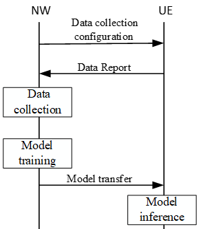
• Core Concept: UE sends measurement data to the network and network trains models.
• Requirements:
  • Uplink bandwidth for measurement reports.
  • Centralized computational resources on the network side.
• Advantages:
  • Models should generalize better across the whole network.
  • Simpler for resource-constrained UEs.

Key Trade-Offs

Which model should be selected ? It depends on several trades-off listed below.

• Overhead vs. Generalization
• Privacy vs. Centralization
• UE Complexity

R1-2400047: Discussion on AIML for CSI prediction

This is about CSI feedback enhancement [RAN1] with a few high level objectives as follows :

• For CSI compression (two-sided model), further study ways to:
• Improve trade-off between performance and complexity/overhead
• e.g., considering extending the spatial/frequency compression to spatial/temporal/frequency compression, cell/site specific models, CSI compression plus prediction (compared to Rel-18 non-AI/ML based approach), etc.
• Alleviate/resolve issues related to inter-vendor training collaboration.
• while addressing other aspects requiring further study/conclusion as captured in the conclusions section of the TR 38.843.
• For CSI prediction (one-sided model), further study performance gain over Rel-18 non-AI/ML based approach and associated complexity, while addressing other aspects requiring further study/conclusion as captured in the conclusions section of the TR 38.843 (e.g., cell/site specific model could be considered to improve performance gain).

Spatial-Temporal-Frequency compression

• Key Points
• AI-based CSI Compression in R18: In the previous 3GPP release (R18), research focused on AI-driven CSI (Channel State Information) compression in the spatial-frequency domain. This involved evaluating performance gains (UPT, SGCS), generalization, and various training collaboration approaches.
• Lack of Consensus: Despite the research, no clear recommendation on CSI compression emerged from a RAN1 (Radio Access Network 1) perspective.
• WID Recommendations: The Workshop on Wireless Innovation and Development (WID) highlighted the need for further exploration of the trade-off between performance and complexity/overhead. They suggested extending compression to spatial/temporal/frequency domains and considering cell/site-specific models or combining compression with prediction.
• Proposed Approach: This contribution proposes AI-based CSI compression in the spatial-temporal-frequency (S-T-F) domain. The idea is to leverage historical CSI data from prior time slots to enhance the compression of current CSI.
• Interpretation & Implications:
• It highlights the ongoing evolution of CSI compression techniques in the context of 5G and beyond.
• Performance vs. Complexity: A core challenge is balancing the benefits of improved compression (reduced overhead, efficient resource utilization) against the increased complexity of AI-based models and potential computational burden.
• Leveraging Temporal Information: The proposed S-T-F compression aims to exploit the inherent correlation between CSI data across time slots. This could lead to more efficient compression algorithms.
• Future Research Directions: The WID recommendations suggest a broader exploration of compression techniques, including adaptation to specific cells or sites and the integration of prediction mechanisms.

< CSI S-T-F compression >

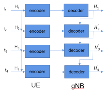
The diagram above depicts a simplified representation of AI-based CSI Spatial-Temporal-Frequency (S-T-F) compression in a wireless communication scenario between a User Equipment (UE) and a gNodeB (gNB). It visually illustrates how AI-based S-T-F compression can be employed in a wireless communication system. By leveraging historical CSI data, the encoder aims to achieve more efficient compression, leading to reduced overhead and improved resource utilization in the network.

• Components and Process:
• H1, H2, H3, H4: These represent CSI (Channel State Information) at different time slots (t1, t2, t3, t4). CSI captures the characteristics of the wireless channel between the UE and gNB, crucial for optimizing transmission.
• Encoder: At the UE side, each CSI (H) is fed into an encoder. The encoder compresses the CSI data, aiming to reduce its size for efficient transmission. Importantly, the encoder likely utilizes historical CSI data (from previous time slots) to enhance the compression of the current CSI. This is the core idea of S-T-F compression - leveraging temporal correlations in CSI.
• Decoder: At the gNB side, the received compressed CSI (H') is passed through a decoder. The decoder reconstructs an estimate of the original CSI data.
• UE and gNB: These represent the two communicating devices in the system. The UE is the user's device (e.g., a smartphone), while the gNB is the base station providing network connectivity.
• Overall Flow:
• CSI Acquisition: The UE measures the CSI of the channel at different time slots.
• Encoding at UE: The CSI data is compressed at the UE using an encoder that exploits both spatial and temporal information (S-T-F compression).
• Transmission: The compressed CSI is transmitted to the gNB.
• Decoding at gNB: The gNB receives the compressed CSI and uses a decoder to reconstruct an estimate of the original CSI.
• Channel Optimization: The gNB utilizes the reconstructed CSI to optimize the communication link (e.g., beamforming, power allocation) to enhance performance and reliability.

Evaluations for CSI S-T-F compression

Overall, this demonstrates the potential of AI-based S-T-F compression for enhancing CSI feedback efficiency in 5G and beyond. Further research could explore other model architectures, optimization techniques, and real-world deployment considerations.

• Model Description
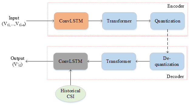
• The diagram shown above visually represents the AI model architecture used for CSI S-T-F (Spatial-Temporal-Frequency) compression, as described in the summary. It showcases a two-sided model consisting of an Encoder and a Decoder, each employing a combination of ConvLSTM and Transformer components.
• Encoder:
• Input: The encoder takes a sequence of historical CSI vectors (V_(t-1), ..., V_(t-n)) as input, where each vector represents the channel state information at a previous time slot.
• ConvLSTM: The ConvLSTM layer processes this input sequence, extracting temporal correlations and features from the historical CSI data.
• Transformer: The Transformer layer, with its multi-head attention mechanism, further compresses the CSI representation from the ConvLSTM, focusing on important spatial relationships.
• Quantization: Finally, the compressed representation is quantized to reduce its bit-width for efficient transmission.
• Decoder:
• De-quantization: The received quantized representation is first de-quantized.
• Transformer: The Transformer layer in the decoder aims to recover the original CSI representation from the compressed and quantized version.
• ConvLSTM: The ConvLSTM layer then leverages the recovered CSI and potentially additional historical CSI information to generate the final estimated CSI output (V_(t)) for the current time slot.
• Historical CSI:
• The green box labeled "Historical CSI" emphasizes the crucial role of past CSI information in both the encoder (for better compression) and potentially the decoder (for improved reconstruction).
• Key Points Illustrated in the Image:
• Two-sided model: The clear separation of encoder and decoder sections highlights the compression and reconstruction phases.
• ConvLSTM for Temporal Features: The use of ConvLSTM layers in both encoder and decoder reflects the importance of capturing temporal dependencies in CSI data.
• Transformer for Compression/Recovery: The presence of Transformer layers underscores their role in compressing and recovering CSI representations using attention mechanisms.
• Quantization/De-quantization: The inclusion of these steps emphasizes the practical aspect of reducing data size for transmission and then restoring it for processing.
• Historical CSI: The separate box highlights how past CSI information is leveraged to enhance both compression and reconstruction processes.

• AI Model for CSI S-T-F Compression
• A two-sided model with encoder and decoder is used for AI-based CSI compression evaluation.
• Encoder: ConvLSTM + Transformer backbone.
• Decoder: Transformer + ConvLSTM backbone.
• ConvLSTM extracts temporal features from past CSI.
• Transformer compresses/recovers current CSI using multi-head attention.
• Evaluation Results for CSI S-T-F Compression
• Dataset: Dense Urban scenario, 2GHz FDD, 1140 UEs, 12 sub-bands.
• Training: 90% training, 10% validation.
• Input: Eigenvector of channel matrix.
• Observation window: 4/5ms for past CSI.
• Metric: SGCS (Spectral Gain Channel Steering)
• Baseline: Rel-16 eType II codebook.
• Results:
• AI-based S-F compression: 4.6%~7% SGCS gain over baseline.
• AI-based S-T-F compression: 8.8%~16.5% SGCS gain over baseline.
• Observations:
• Both AI-based methods outperform the baseline.
• S-T-F compression provides significantly higher SGCS gain than S-F.
• Relative SGCS gain decreases as the number of feedback bits increases.
• Interpretation:
• The proposed AI model for S-T-F compression effectively leverages temporal correlations in CSI data, leading to superior performance compared to S-F compression and the traditional codebook.
• The use of ConvLSTM for temporal feature extraction and Transformer for compression/recovery seems to be a successful combination.
• The diminishing relative gain with increased feedback bits suggests that there's a limit to how much improvement AI can provide as more information is available.

R1-2400094: Discussion on other aspects of AI/ML model and data on AI/ML for NR air-interface

Overview of this documents are as follows :

• Focus: Integration of AI/ML into the NR air-interface, building on previous discussions.
• Key Topics:
• Necessity and types of model identification (offline, over-the-air signaling)
• Additional conditions for AI/ML model training and inference (network-side and UE-side)
• Model transfer/delivery mechanisms
• Proposals:
• Clarifications on model identification processes (Type B1 and B2)
• Network control over model ID assignment
• UE capability reports for indicating supported models
• Identification and justification of additional conditions for each use case
• Adoption of a transparent approach (e.g., OTT) for model transfer/delivery

Model Identification Type

In the context of AI/ML model integration for the NR air-interface, the necessity and specifics of model identification are under scrutiny, particularly concerning its role in Lifecycle Management (LCM). This discussion is crucial as it impacts how models are managed, updated, and utilized within the network. The distinction between offline and over-the-air identification methods is also being explored, along with the potential implications for standardization and interoperability.

Followings are summary of model identification types discussed in this document : (Some of the keywords (e.g, Type A, B etc) will pop out frequently in other documents, so better to get familiar with them)

• Model Identification Types
• Type A:
• Model identification occurs without over-the-air signaling.
• A model ID may be assigned during identification for later use in over-the-air signaling.
• Specification impact on other WGs needs further study.
• Type B:
• Model identification happens through over-the-air signaling.
• Type B1:
• Initiated by the UE, with NW assistance in remaining steps.
• A model ID may be assigned during identification.
• Details of the steps involved require further study.
• Type B2:
• Initiated by the NW, with UE response in remaining steps.
• A model ID may be assigned during identification.
• Details of the steps involved require further study.
• Further Clarifications and Proposals
• Example use cases for Type B1 and B2:
• Model identification during model transfer from NW to UE
• Model identification related to data collection configurations, indications, or dataset transfer
• Other use cases are not excluded
• Offline model identification might apply to some of these cases
• Unclear points requiring further study:
• How UE initiates and NW assists in Type B1
• How NW initiates and UE responds in Type B2
• The specific "remaining steps" in both types
• The entity responsible for assigning model IDs (Proposal: NW should have control)

R1-2400095: Discussion on potential performance enhancements/overhead reduction with AI/ML-based CSI feedback compression

The purpose of this document is to discuss potential performance enhancements and methods for reducing overhead in AI/ML-based CSI feedback compression, particularly for the two-sided model use case in NR (New Radio). The focus is on improving the trade-off between performance and complexity in AI/ML-based CSI compression compared to earlier non-AI/ML methods like the Rel-16 eType II codebook-based approach.

Followings are summary of this document :

• Rel-18 Study Observations:
• AI/ML-based CSI compression shows significant CSI feedback overhead reduction compared to traditional methods (Rel-16 eType II codebook-based).
• The gain in mean UPT (User Plane Throughput) using AI/ML is moderate.
• Performance gain increases with higher RU (Resource Utilization).
• AI/ML achieves considerable amount of CSI feedback overhead reduction depending on max rank and traffic type (Ref TR 38.843).
• Performance Improvement Options:
• Temporal-domain information: Including temporal aspects in addition to spatial-frequency information for CSI compression.
• Joint CSI compression and prediction: Combining compression and prediction for potential gains, but requires further study on NW-side (Network-side) CSI prediction performance.
• Cell/site-specific models: Using models tailored to specific cells or sites instead of generalized models.
• CSI Feedback Overhead Reduction:
• CSI LUT (Look-Up Table)-based approach: A vector quantization method where the optimal CSI codebook entry is selected and its index is sent as feedback.
• Advantages of LUT:
• Can achieve the performance upper bound of typical VQ (Vector Quantization)-based approaches.
• Outperforms VQ in SGCS (Squared Generalized Cosine Similarity?) and reduces CSI feedback overhead significantly while maintaining similar mean UPT.
• Offers a good balance between performance gain and complexity.
• Observation: AI/ML with LUT and 26 bits overhead achieves similar mean UPT as Rel-16 with ~155 bits overhead ( ~83% reduction, Ref : Table 2.2-1).
• The document proposes to consider CSI LUT for Rel-19 to balance performance and complexity trade-offs.
• Leveraging Temporal-Domain Information:
• Potential for further improvement: Using temporal attributes in addition to spatial-frequency information as input to the AI/ML model.
• Initial performance comparison: SFT (Spatial-Frequency-Temporal) compression outperforms SF (Spatial-Frequency) compression in SGCS consistently.
• Observation: SFT shows ~11-12% SGCS gain over SF with LUT-based quantization(Table 2.3-1).

R1-2400146: Discussion on CSI prediction for AI/ML

One thing that I want to note from this document is the potential specification impacts of integrating AI/ML-based CSI prediction, such as performance monitoring, data collection, and functionality fallback mechanisms.

Performance Monitoring Approaches for UE-Side CSI Prediction in Functionality-Based Lifecycle Management

As an agreed item is three types of performance monitoring approaches have been proposed by companies to facilitate functionality-based lifecycle management (LCM) for CSI prediction using the UE side model

• Type 1: The UE calculates the performance metrics and reports the monitoring output to the network and then the network can  make decisions on functionality fallback to legacy CSI reporting. The network may also set a threshold criterion for the UE's performance monitoring.
• UE calculate the performance metric(s)
• UE reports performance monitoring output that facilitates functionality fallback decision at the network
• Performance monitoring output details can be further defined
• NW may configure threshold criterion to facilitate UE side performance monitoring (if needed).
• NW makes decision(s) of functionality fallback operation (fallback mechanism to legacy CSI reporting).
• Type 2: The UE reports both the predicted CSI and the ground truth to the network and then the network calculates the performance metrics and decides on any fallback operation to legacy CSI reporting.
• UE reports predicted CSI and/or the corresponding ground truth  
• NW calculates the performance metrics.
• NW makes decision(s) of functionality fallback operation (fallback mechanism to legacy CSI reporting)
• Type 3: Similar to Type 1, the UE calculates the performance metrics and reports them to the network and then the network decides on fallback operations.
• UE calculate the performance metric(s)
• UE report performance metric(s) to the NW
• NW makes decision(s) of functionality fallback operation (fallback mechanism to legacy CSI reporting).

Further clarifications.

It would not seem to be so clear just by reading the definition from the document(at least seems ambiguous to me). So let's try rewrite the definition in a little bit difference structure

Common to All

Followings are the factors / functionality that would apply to all types

• UE Involvement in Performance Metrics: In all three types, the UE is responsible for either calculating or reporting performance metrics, which are used to assess the accuracy or effectiveness of the AI/ML-based CSI prediction.
• Network Decision Making: In each type, the network ultimately decides on the actions related to functionality control, such as whether to activate or fall back to legacy reporting, based on the data received from the UE.
• Functionality Fallback to Legacy CSI Reporting: All types involve a mechanism where the network (NW) makes decisions about falling back to legacy CSI reporting based on the performance metrics.
• Configurable CSI-RS and Performance Monitoring Procedures: All types rely on CSI-RS configuration and have procedures in place for performance monitoring, which can include periodic, semi-persistent, or event-driven reporting.
• Intermediate KPIs (e.g., NMSE, SGCS): Each type of monitoring uses intermediate performance metrics, such as NMSE (Normalized Mean Squared Error) or SGCS (Subband Gain Computation Score), to evaluate the system's functionality.
• Potential Reuse of Existing Functionality Selection Mechanisms: Across all three types, the existing mechanisms for selecting, activating, deactivating, or switching UE functionality may be reused, if applicable.

Differences among types

Main differences among types are from the type of the contents that UE reports to the network.

• Type 1: the UE reports performance monitoring output, not raw CSI data.
• The UE calculates the performance metrics itself and reports the performance monitoring output to the network (NW).
• The UE does not directly report the predicted CSI or the ground truth, but instead, it reports whether the AI/ML model is performing well based on predefined criteria (like a threshold).
• The network then decides on functionality fallback based on the output provided by the UE.
• Type 2 the UE reports both the predicted and ground truth CSI to the network, leaving the calculation of metrics to the network
• The UE reports both the predicted CSI and/or the corresponding ground truth CSI to the network.
• The network is responsible for calculating the performance metrics using the reported data.
• Based on the metrics, the network makes decisions regarding functionality fallback.
• Type 3: the UE calculates and reports performance metrics to the network, but does not report raw CSI data.
• The UE calculates the performance metrics (similar to Type 1) but directly reports these metrics to the network.
• The network uses these reported metrics to decide on any fallback actions, but the UE doesn't provide the predicted or ground truth CSI directly.

Data Collection

For CSI prediction, the model input is channel information from the UE. The UE measures the DL channel and performs model inference autonomously. The model output, either channel matrix or precoding matrix, can be converted to legacy codebooks. For data collection for model training, the UE measures the DL channel and generates training data. The UE may or may not need to report the predicted CSI, depending on whether there is traffic.

The mechanism of Rel-18 MIMO may be reused for the configuration of CSI measurement and report for AI/ML based CSI prediction. The functionality based LCM of UE side model of BM can be reused for the functionality based LCM for AI/ML based CSI prediction. The indication of assistance information/additional condition from NW to UE is considered with low priority unless clear motivation is justified.

Key points :

• The model inference for CSI prediction can be performed autonomously by the UE based on existing configurations.
• Training data can be gathered even in the absence of traffic, with ground-truth CSI acquired through specific gNB indications.
• The network side's assistance information is deemed of low priority unless it serves a justified purpose.

Model Inference:

• The model input for CSI (Channel State Information) prediction is channel data measured by the UE, such as channel matrix or precoding matrix.
• The UE measures the DL channel and performs inference autonomously using the configured CSI-RS resources.
• The model's output, regardless of its form, can be converted to legacy codebooks. For multi-time instance outputs, the Rel-18 Doppler codebook can compress the predicted CSI.
• If the CSI-RS configuration doesn’t align with the model’s input requirements, the UE can either fall back to non-prediction mode or request the gNB to reconfigure the parameters.

Model Training:

• The UE can autonomously generate training data using the configured CSI-RS resources and measure the DL channel within the observation window.
• If there’s no traffic, the UE may choose not to report the predicted CSI, preserving it only for training purposes.
• Ground-truth CSI can be obtained by linking prediction reports with ground-truth reports, facilitated by gNB indications.

Performance Monitoring

Three types of performance monitoring procedures(Type 1,2,3) are discussed, with the main differences being the roles of the UE and NW in calculating performance metrics and making decisions.

For all three types, the UE needs to be configured with CSI-RS resource and CSI report for both predicted CSI and ground-truth CSI. The UE may also need to be indicated with the association between predicted CSI and the measurement of ground-truth CSI.

Overall, the main difference lies in where the performance metrics are calculated and how decisions are made based on those metrics. Type 1 involves the UE calculating metrics and the NW making decisions based on the UE's monitoring outputs. Type 2 involves the UE reporting data and the NW calculating metrics and making decisions. Type 3 involves the UE calculating metrics and the NW making decisions based on those metrics.

Monitoring Types Overview:

There are three types of monitoring procedures, with the main differences being the roles of the UE and NW (network) in calculating performance metrics and making decisions.

Type 1:

• The UE calculates performance metrics and compares them against a threshold criterion.
• If metrics indicate good performance, the model continues operation. Otherwise, it may not meet inference requirements.
• The threshold criterion could use metrics like the SGCS and the output can suggest actions like activation or fallback.
• The network takes the UE’s report as a reference to decide whether to command functionality changes.

Type 2:

• The UE does not perform calculations but reports the AI/ML output and a ground-truth label to the network.
• Possible ground-truth labels include:
• Channel Matrix: Directly reflects the model’s output but has high reporting overhead.
• Legacy Codebook/PMI (Precoding Matrix Indicator): Simplifies reporting by converting the channel matrix to PMI, making it easier for the network to derive metrics.
• The network calculates performance metrics based on the reported data and decides on necessary actions.

Type 3:

• Similar to Type 1, the UE calculates performance metrics (e.g., SGCS) and may use statistical values over a monitoring window.
• The network uses the metrics to make decisions on actions like activation or fallback.
• Common Aspects for All Types:
• All three types involve configuration of CSI-RS resources and reporting of both predicted and ground-truth CSI.
• UE may need to associate predicted CSI with ground-truth CSI measurements if the CSI-RS resource for ground-truth is not in the same slot as the predicted CSI but in a neighboring slot.
• This association is necessary for the network to understand and evaluate the model’s performance.

Summary:

• Type 1 focuses on UE-side calculations with the network taking actions based on UE reports.
• Type 2 shifts calculation responsibility to the network, with the UE providing raw data and labels.
• Type 3 is similar to Type 1 but emphasizes statistical value monitoring over a specific window.
• Regardless of type, proper configuration and association of CSI-RS resources are crucial for accurate performance monitoring.

R1-2400150: Discussion on CSI compression for AI/ML

The document focuses on the discussion of CSI (Channel State Information) compression for AI/ML (Artificial Intelligence/Machine Learning) in the context of 5G NR (New Radio). It explores ways to enhance CSI compression techniques using AI/ML, addressing challenges related to performance, complexity, inter-vendor collaboration, and other open issues from previous releases (like Rel-18).

Specifically, the document delves into:

• Extending CSI compression to the temporal-spatial-frequency (TSF) domain: This involves leveraging temporal correlations in channel measurements to improve compression efficiency. It discusses AI/ML model descriptions, simulation assumptions, preliminary results, complexity alleviation techniques, and potential specification impacts.
• Extending CSI compression to cell/site-specific models: This explores the possibility of tailoring CSI compression models to specific cells or sites to enhance performance. It discusses evaluation methodologies, potential specification impacts, and challenges related to channel modeling and avoiding overfitting.
• Extending CSI compression to CSI compression plus CSI prediction: This investigates combining CSI compression with CSI prediction to further improve overall efficiency. It discusses evaluation methodologies, potential specification impacts, and the applicability of this approach to specific scenarios.
• Inter-vendor training collaboration: It addresses challenges related to collaboration between different vendors in training AI/ML models for CSI compression. It discusses different types of training collaborations, their pros and cons, and proposes prioritizing certain approaches.
• Other aspects with respect to further studies: It continues discussions on open issues from Rel-18, including data collection, monitoring, and CSI inference aspects. It proposes specific approaches and considerations for each of these aspects.

NOTE : Main reason why I am personally personally interested in this document is the technical details about the AI/ML model. For this summary note, I would focus more on the details on AI/ML model.

R1-2500051 : Discussion of CSI compression on AI/ML for NR air interface

In this document, a lot of agreements across the entire scope of CSI compression are well summarized.

Inter-vendor training collaboration options/directions

This is for inter-vendor collaboration on AI/ML-based CSI (Channel State Information) feedback and precoding models for 5G/6G networks. It discusses agreements on the feasibility and standardization of scalable model structures for CSI feedback and precoding across multiple vendors.

• Agreement
• •For Direction A Option 3a-1 and Direction C, study the feasibility of scalable model structure specification over numbers of Tx ports, CSI feedback payload sizes, and bandwidths, number of slots.
• Feasibility of Direction A Option 3a-1 is contingent on the feasibility of the scalable model structure specification.
• Feasibility of Direction C is contingent on the feasibility of the scalable model structure specification and model parameters specification.
• Note: Angular/Delay/Doppler domain conversion and quantization are considered to be part of feasibility study.
• Agreement
• For studying the standardized model structure,
• For temporal domain Case 0,
• In case of spatial-frequency domain input, adopt Transformer as the backbone structure.
• Further study angular-frequency and angular-delay domain input
• For temporal domain Case 2,
• In case of spatial-frequency domain input, take into account the model structure of Case 0 with an adaptation. Study the following options for the adaptation:
• Option 1: Input/output adaptation with additional layers
• Conv-LSTM
• LSTM
• Option 2: Latent adaptation on top of Case 0 model structure
• Reusing Case 0 structure and changing quantization operation and/or feedback payload over different slots
• Note: other options are not precluded
• Further study angular-frequency and angular-delay domain input
• For temporal domain Case 3,
• In case of spatial-frequency domain input, take into account the model structure of Case 0 with an adaptation. Study the following options for the adaptation:
• Option 1: Input/output adaptation
• Option 2: Latent adaptation
• Further study angular-frequency, angular-delay, and angular-delay-Doppler domain input.
• Take precoding matrix in the spatial-frequency domain in a subband granularity as the input, and the reconstructed precoding matrix in the spatial-frequency as the output, for the study of standardized model structure.
• Note: Processing steps at the UE to derive angular, delay, and/or Doppler domain basis, and corresponding reconstruction steps at the gNB are considered.
• Note: scalar/vector quantization and dequantization are considered. Quantization-aware training with jointly updated quantization method/parameters (Case 2-2) is used.

High level implication of these agreement can be stated as follows :

• Collaboration for Standardization – This document outlines how different vendors can collaborate on standardizing AI/ML-based CSI feedback and precoding methods, ensuring interoperability and efficiency across different network configurations.
• Scalability of AI Models – It emphasizes the scalability of model structures for different 5G/6G parameters, acknowledging the need for adaptable AI architectures that can dynamically adjust to variations in the number of transmission ports, feedback payload sizes, bandwidths, and slot configurations. Given the complexity of real-world network deployments, the ability to generalize across these parameters is critical for enabling a flexible and efficient CSI feedback mechanism that can operate seamlessly across various environments.
• AI Models for CSI Feedback – The study also focuses on the use of AI models, particularly Transformers, LSTMs, and Conv-LSTMs, as core architectures for processing CSI feedback and precoding tasks. Transformers, known for their ability to capture long-range dependencies and complex spatial-frequency patterns, serve as the primary backbone structure for handling CSI feedback. Meanwhile, LSTMs and Conv-LSTMs provide temporal modeling capabilities, enabling efficient adaptation over time by incorporating memory mechanisms that help track changes in the wireless channel. These models are explored within different temporal domain cases to determine their effectiveness in enhancing CSI compression and reconstruction, ensuring that AI-driven feedback mechanisms remain both computationally efficient and robust against dynamic network conditions.
• Feasibility of Domain Transformations – Feasibility studies are also conducted to assess the incorporation of different domain transformations, including angular, delay, and Doppler domains, in AI-based CSI processing. Given that CSI can be represented in multiple mathematical domains depending on transmission characteristics, exploring these transformations helps in optimizing feedback accuracy and reducing overhead. Angular domain transformations improve spatial resolution for beamforming applications, delay domain transformations enhance time-domain analysis for multipath-rich environments, and Doppler domain transformations aid in characterizing mobility effects for high-speed scenarios. By evaluating the feasibility of AI models operating in these domains, the study ensures that standardized CSI feedback techniques can support a diverse range of deployment scenarios, including those in dense urban environments, high-mobility networks, and massive MIMO systems.
• Efficient Quantization Techniques – Another crucial aspect of this collaboration involves quantization techniques for efficient feedback, addressing the need to reduce feedback overhead while preserving the integrity of CSI information. Since transmitting raw CSI feedback requires significant bandwidth, effective quantization methods are necessary to enable compression while maintaining signal quality. The study examines both scalar and vector quantization approaches, incorporating quantization-aware training methods that allow AI models to jointly optimize CSI representation and compression techniques. Adaptive quantization strategies are also explored to allow CSI feedback mechanisms to dynamically adjust quantization levels based on network conditions, ensuring that the feedback remains efficient without compromising accuracy.
• Towards AI-Enhanced 5G/6G Networks – Through these efforts, the document sets the foundation for a standardized, AI-enhanced CSI feedback and precoding framework that can be universally adopted across vendors, contributing to the broader goal of enhancing wireless network performance in 5G and future 6G deployments.

LCM aspects

This outlines an agreement related to LCM aspects in the context of temporal domain Case 3, focusing on data collection methods for training and monitoring CSI (Channel State Information) prediction and compression.

• Agreement
• For temporal domain aspects Case 3, study LCM aspects and specification impacts,
• consider the following options for training data collection
• Option 1: The target CSI for training is derived based on the predicted CSI of the future slot(s).
• Option 2: The target CSI for training is derived based on the measured CSI of the future slot(s).
• Note: During inference, the input to the CSI generation part is derived based on the predicted CSI.
• consider following options for the monitoring labels
• Option 1: The monitoring label is derived based on the predicted CSI of the future slot(s).
• CSI prediction output is used as input to CSI generation part.
• Note: This corresponds to monitoring of CSI compression only. CSI prediction may be monitored separately.
• Option 2: The monitoring label is derived based on the measured CSI of the future slot(s)
• Option 2a: CSI prediction output is used as input to CSI generation part.
• Note: This corresponds to end-to-end monitoring of CSI prediction and compression.
• Option 2b: Measured CSI of the future slot(s) is used as input to CSI generation part for monitoring purpose.
• Note: This corresponds to monitoring of CSI compression only. CSI prediction may be monitored separately.
• Study how the functionality/model control (activation, deactivation, switching, and fallback) for CSI prediction and CSI compression interacts.

The agreement centers on LCM (Lifecycle Management) aspects within the context of temporal domain Case 3, specifically addressing data collection strategies for training and monitoring CSI (Channel State Information) prediction and compression.

• Training Data Collection Strategies – Two approaches are considered for deriving the target CSI for training: one based on the predicted CSI of future slots and another based on the measured CSI of future slots. The input to the CSI generation model during inference is derived from predicted CSI.
• Options for Monitoring Labels – The agreement explores two methods for monitoring labels. The first method derives the monitoring label from predicted CSI, which primarily enables monitoring of CSI compression separately from prediction. The second method derives the monitoring label from measured CSI, allowing for end-to-end monitoring of CSI prediction and compression.
• Implications of Predicted vs. Measured CSI – Using predicted CSI focuses on monitoring compression efficiency without directly assessing prediction accuracy, whereas using measured CSI allows for a complete evaluation of both prediction and compression. Measured CSI also serves as an input for CSI generation to facilitate monitoring.
• End-to-End Monitoring in Option 2a – When measured CSI is used as a monitoring label and the CSI prediction output is used as an input for CSI generation, this enables a comprehensive monitoring approach that evaluates the full CSI feedback pipeline, including both prediction and compression.
• Separate Monitoring in Option 2b – Another approach considers measured CSI solely for monitoring purposes, without incorporating prediction output into the CSI generation process. This method is focused exclusively on monitoring the effectiveness of CSI compression while treating CSI prediction as a separate entity.
• Interaction Between CSI Prediction and Compression – The agreement emphasizes the importance of studying how CSI prediction and CSI compression interact, as optimizing one can influence the performance of the other. Understanding this relationship is crucial for designing an efficient CSI feedback mechanism.
• Functionality and Model Control – Various aspects of model control are considered, including activation, deactivation, switching, and fallback mechanisms. These controls ensure that the CSI prediction and compression models can dynamically adapt to network conditions, improving efficiency and robustness.
• Impact of Model Switching – The agreement recognizes that switching between models or configurations can affect CSI feedback performance. Evaluating how transitions between different models impact prediction accuracy and compression efficiency is a key part of the study.
• Relevance to 5G/6G Networks – By defining standardized approaches for training, monitoring, and controlling CSI prediction and compression, this agreement contributes to optimizing CSI feedback mechanisms in future wireless networks. These efforts will help enhance the efficiency and scalability of AI-based CSI feedback solutions in 5G and 6G deployments.

Data collection at NW-side and UE-side

This outlines an agreement related to Data collection at NW-side and UE-side

• Agreement
• For NW to collect data for training, study following spec impacts
• •Data format: codebook-based Rel-16 eType2 or Rel-18 eType2 for PMI prediction.
• FFS if enhancement is needed
• FFS number of samples in the report.
• FFS whether channel or precoder is needed for temporal Cases 3
• Configuration of rank/layer, number of subbands
• Mechanism for ground-truth reporting
• FFS: Report additional information regarding the samples, e.g., data quality, FFS the definition of data quality and corresponding parameters.
• FFS if enhancements in CSI-RS and SRS configuration is needed.
• FFS: Report associated information that captures UE side additional condition
• FFS: Configuration / reporting of temporal aspects for temporal Case 2 and Case 3, e.g., association between input and output CSI
• FFS: details of CSI measurement
• For UE to collect data for training, study following spec impacts
• NW configuration or UE request, e.g., RS configuration/transmission for data collection
• Whether enhancements in CSI-RS configuration is needed.
• Configuration of temporal aspects for temporal case 2/3, e.g., association between input and output CSI
• FFS: Need of configuration of ID, and configuration of ID

This agreement defines the requirements and specifications for data collection at both the network (NW) side and the UE side to facilitate training processes for CSI (Channel State Information) prediction and related AI-based processing.

• NW-Side Data Collection for Training – The agreement specifies various considerations for the network side when collecting training data. The data format should support codebook-based Rel-16 eType2 or Rel-18 eType2 for PMI (Precoder Matrix Indicator) prediction. Additional enhancements in feedback frequency selection (FFS), including the number of samples in reports, are considered. The need for precoder inclusion in temporal Case 3 is also assessed. Further aspects include rank/layer configuration, number of subbands, and ground-truth reporting mechanisms. The report must capture additional details, including data quality, CSI-RS and SRS enhancements, UE-side conditions, temporal associations between input and output CSI, and specific CSI measurement details.
• UE-Side Data Collection for Training – On the UE side, the agreement outlines specifications for data collection requirements. It includes whether RS (Reference Signal) configuration and transmission should be determined by NW configuration or UE request. The study also examines whether CSI-RS enhancements are required for better data collection. Additionally, the configuration of temporal aspects for Case 2 and Case 3 is analyzed, particularly how input and output CSI are associated. The agreement also highlights the need for ID configuration to ensure proper data tracking and management.
• Standardization and Future Optimization – The structured approach to defining network-side and UE-side data collection mechanisms plays a critical role in optimizing AI-based CSI prediction and feedback mechanisms. By ensuring well-defined data structures, configurations, and reporting formats, this effort contributes to improving training data quality and facilitating interoperability across different network deployments in 5G and beyond.

UE-side/NW-side data distribution mismatch

This outlines an agreement related to UE-side/NW-side data distribution mismatch

• Agreement
• For discussion on performance degradation due to UE-side / NW-side data distribution mismatch with respect to UE side additional condition (issue 4 and 6), consider
• NW-side data (dataset A) and UE-side data (dataset B) are mismatched in terms of UE-side additional condition (e.g., SVD phase normalization method, UE antenna virtualization, antenna imbalance, antenna spacing / layout, etc)
• Note: dataset A may or may not contain dataset B
• Note: if dataset A includes dataset B, this means NW timely collect data from the UE
• Note: Dataset A and dataset B are aligned in terms of NW-side additional conditions.
• Case 1: An encoder-decoder pair is trained on dataset B. This serves as an upper-bound.
• Case 2 (for direction A):
• For direction A: NW-side trains a decoder on dataset A, and UE-side trains an encoder based on either dataset A, dataset B, or both (where the choice depends on the inter-vendor collaboration Options (4-1 or 3a-1), the training alternatives (Alt 1 or Alt 2) within the Options, and the choice of target CSI for training)
• Case 3 (for direction B): NW-side train an encoder-decoder on dataset A and transfers the encoder parameters to UE.
• Study issue 4 and 6 by evaluating the inference performance for Case 2 / 3 on test dataset B, comparing to the inference performance for case 1 on test dataset B.
• Note: Evaluations are assumed to performed without common reference model structure among companies

• Agreement
• Direction C: Fully standardized reference model(s) and parameters with specified CSI generation part and/or CSI reconstruction part (Inter vendor collaboration option 1), including at least the following issues
• [Issue 9] Is there performance impact due to mismatch between the distribution of the dataset used for reference model(s) training, UE-side data distribution, and NW-side data distribution, and if so, how to address it?

The agreement focuses on the potential performance degradation caused by mismatches between UE-side and NW-side data distributions in CSI feedback and reconstruction. These mismatches arise due to UE-side additional conditions, including variations in SVD phase normalization methods, UE antenna virtualization, antenna imbalance, and antenna spacing/layout. Understanding the impact of such mismatches is crucial for improving CSI prediction models.

• Definition of Dataset A and Dataset B – The agreement considers two datasets:
• Dataset A represents NW-side data, which may or may not include dataset B.
• Dataset B consists of UE-side collected data, ensuring alignment in terms of NW-side additional conditions.
• If dataset A includes dataset B, it means the NW collects data directly from the UE.
• Training Approaches for Addressing Mismatch –
• Case 1 defines a baseline where an encoder-decoder pair is trained directly on dataset B, establishing an upper-bound reference.
• Case 2 (Direction A) involves NW-side training a decoder on dataset A, while UE-side trains an encoder based on dataset A, dataset B, or a combination of both. The selection of training datasets depends on inter-vendor collaboration options (e.g., 4-1 or 3a-1) and the choice of target CSI for training.
• Case 3 (Direction B) follows a different approach where NW-side trains an encoder-decoder on dataset A and transfers the trained encoder parameters to the UE, allowing the UE to benefit from NW-side training.
• Evaluation of Training Performance – The agreement includes a study on issues 4 and 6, where the inference performance of Case 2 and Case 3 on test dataset B is compared against Case 1 performance on test dataset B. This ensures that the proposed approaches effectively mitigate performance degradation due to distribution mismatches. Evaluations assume no common reference model structure across different companies, making interoperability an essential factor.
• Direction C: Standardized Reference Models for CSI Generation – The agreement also includes Direction C, which aims to establish fully standardized reference models and parameters for CSI generation and reconstruction, ensuring alignment across vendors. A key issue (Issue 9) addresses whether the dataset mismatch between reference model training, UE-side data distribution, and NW-side data distribution impacts performance. If so, solutions to mitigate these discrepancies need to be developed.
• Objective for Standardization – By addressing UE-side/NW-side data distribution mismatches, this agreement aims to improve generalization, robustness, and efficiency in CSI feedback and reconstruction, ultimately benefiting interoperability and performance optimization in AI-based CSI processing for 5G and future 6G networks.

Specification impacted related to inter-vendor training collaboration

This outlines an agreement related to Specification impacted related to inter-vendor training collaboration

• Agreement
• For Direction A Option 3a-1 and Direction C, study the feasibility of scalable model structure specification over numbers of Tx ports, CSI feedback payload sizes, and bandwidths, number of slots.
• Feasibility of Direction A Option 3a-1 is contingent on the feasibility of the scalable model structure specification.
• Feasibility of Direction C is contingent on the feasibility of the scalable model structure specification and model parameters specification.
• Note: Angular/Delay/Doppler domain conversion and quantization are considered to be part of feasibility study.

The agreement emphasizes studying the feasibility of a scalable model structure specification for inter-vendor training, ensuring that AI-based CSI feedback models can adapt across various Tx ports, CSI feedback payload sizes, bandwidths, and slot configurations.

• Dependency of Direction A Option 3a-1 – The feasibility of Direction A Option 3a-1 is entirely dependent on whether a scalable model structure can be effectively designed. Without a standardized and adaptable framework, this option cannot be implemented efficiently across different network setups.
• Dependency of Direction C – The feasibility of Direction C not only depends on the scalable model structure but also on the specification of model parameters, ensuring that AI models trained across different vendors can achieve consistency and interoperability.
• Inclusion of Domain Conversion & Quantization – The feasibility study will also cover angular, delay, and Doppler domain conversion, along with quantization techniques. These factors are critical in improving CSI feedback efficiency, reducing overhead, and ensuring robust performance in dynamic 5G/6G network environments.
• Objective of Standardization – By defining a scalable and interoperable model structure, this agreement aims to facilitate seamless AI-based CSI training and deployment across multiple vendors, ultimately enhancing CSI feedback and precoding efficiency in next-generation wireless networks.

Parameter/model exchange and dataset exchange

This outlines an agreement related to Parameter/model exchange and dataset exchange

• Agreement
• For Directions of addressing inter-vendor collaboration complexity for two-sided CSI compression,
• For Direction A:
• Further study the following options with potential down-selection
• 4-1: dataset is {target CSI, CSI feedback},
• 3a-1: encoder parameter exchange, with {target CSI}
• Note: Additional information beyond what’s listed above may need to be exchanged if necessary.

• Agreement
• For issues listed for inter-vendor collaboration direction B, further study the overhead in Direction B based on the size of the encoder (i.e., number of parameters and quantization level), the number of encoders, and how often the parameters need to be transferred.

• Conclusion
• Standardized signalling, if feasible and specified, can be used for parameter / model exchange in option 3a/5a and 3b to alleviate/resolve the inter-vendor training collaboration complexity.
• Standardized signalling may be reused for exchanging CSI generation part, CSI reconstruction part, or both, etc, when necessary and feasible.
• Standarized signalling may be over-the-air, or other approaches.
• Standardized signalling, if feasible and specified, can be used for dataset exchange in option 4 to alleviate/resolve the inter-vendor training collaboration complexity.
• Standardized signalling may be reused for dataset exchanging, when necessary and feasible.
• Standardized signalling may be over-the-air, or other approaches.
• Note: feasibility will be discussed separately.

The agreement focuses on addressing the complexity of inter-vendor collaboration in two-sided CSI compression. It considers different exchange mechanisms to facilitate efficient data sharing between vendors.

• Dataset and Parameter Exchange in Direction A – Two key options are explored for enabling collaboration in Direction A:
• Option 4-1: Exchanging datasets, which include target CSI and CSI feedback.
• Option 3a-1: Exchanging encoder parameters while sharing target CSI to ensure compatibility between vendor implementations.
• Additional information may be exchanged beyond these listed options when necessary.
• Overhead Considerations in Direction B – The agreement highlights the need to study the overhead associated with Direction B, particularly focusing on the encoder size, which includes factors like the number of parameters and quantization levels. It also considers the number of encoders involved and how frequently parameters must be exchanged. These factors influence the feasibility and efficiency of inter-vendor collaboration.
• Standardized Signaling for Model and Dataset Exchange – The conclusion emphasizes the potential use of standardized signaling to simplify parameter and dataset exchange:
• For model/parameter exchange (Option 3a/5a and 3b): Standardized signaling can help transfer CSI generation and reconstruction parameters between vendors in a structured and efficient way.
• For dataset exchange (Option 4): Standardized signaling could be reused for dataset sharing, reducing inter-vendor complexity.
• Flexible Transmission Methods: The agreement allows for over-the-air transmission or other approaches, depending on feasibility.
• Future Considerations – The feasibility of standardized signaling for both parameter and dataset exchange will be studied further to determine its practicality for inter-vendor training collaboration. This work is expected to enhance the scalability and efficiency of AI-driven CSI feedback mechanisms in 5G/6G networks.

Reference

• 3GPP TR/TS/General
• 3GPP - Finding AI in 3GPP
• 3GPP - RAN3 completes AI & ML support study
• 3GPP - AI/ML for NR Air Interface
• 3GPP TR 22.874 - Study on traffic characteristics and performance requirements for AI/ML model transfer in 5GS (Release 18)
• 3GPP TR 22.875 - Study on AI/MLModel Transfer Phase 2
• 3GPP TR 23.700-80 Study on 5G System Support for AI/ML-based Services (Release 18)
• 3GPP TR 23.700-91 Study on enablers for network automation for the 5G System (5GS); Phase 2 (Release 17)
• 3GPP TR 28.908 Study on Artificial Intelligence / Machine Learning (AI/ML) management (Release 18)
• 3GPP TR 33.852 - Study on traffic characteristics and performance requirements for AI/ML model transfer in 5G Systems (5GS)
• 3GPP TR 33.898 - Study on security and privacy of Artificial Intelligence/Machine Learning (AI/ML)-based services and applications in 5G
• 3GPP TR 37.817 - Study on enhancement for Data Collection for NR and EN-DC
• 3GPP TR 38.843 - Study on Artificial Intelligence (AI)/Machine Learning (ML) for NR air interface
• 3GPP TS 28 105 Artificial Intelligence/ Machine Learning (AI/ML) management
• 3GPP TS 28.550 - Management and orchestration; Performance assurance
• 3GPP RP-221348 Study on Artificial Intelligence (AI)/Machine Learning (ML) for NR Air Interface
• 3GPP R1-2204060 3GPP TSG RAN WG1  #109-e e-Meeting, Beam management with AI/ML
• 3GPP TSG RAN WG1 Meeting #109-e : Discussions on other potential use cases of AI/ML for NR air interface
• 3GPP TR 38.843 V18.0.0 (2023-12) - Study on Artificial Intelligence (AI)/Machine Learning (ML) for NR air interface(Release 18)
• 3GPP R1-2204060 3GPP TSG RAN WG1  #109-e e-Meeting, Beam management with AI/ML
• 3GPP R1-2204571 - Evaluation on ML for CSI feedback enhancement (May 2022)
• 3GPP TDocs
• TSG RAN WG1 #116
• R1-2401766 : Session notes for 9.1 (Artificial Intelligence (AI)/Machine Learning (ML) for NR Air Interface) - TSG RAN WG1 #116  February 26th March 1st, 2024
• R1-2401599 - FL summary #3 for AI/ML in management : 3GPP TSG RAN WG1 #116 - February 26th March 1st, 2024
• R1-2401598 : FL summary #1 for AI/ML in management - 3GPP TSG RAN WG1 #116 February 26th March 1st, 2024
• R1-2401597 : FL summary #1 for AI/ML in management - 3GPP TSG RAN WG1 #116 February 26th March 1st, 2024
• R1-2401596 : FL summary #1 for AI/ML in management - 3GPP TSG RAN WG1 #116 February 26th March 1st, 2024
• R1-2401573 : Final Summary for other aspects of AI/ML model and data - 3GPP TSG RAN WG1 #116 February 26th March 1st, 2024
• R1-2401572 : Summary #4 for other aspects of AI/ML model and data - 3GPP TSG RAN WG1 #116 February 26th March 1st, 2024
• R1-2401571 : Summary #3 for other aspects of AI/ML model and data - 3GPP TSG RAN WG1 #116 February 26th March 1st, 2024
• R1-2401570 : Summary #2 for other aspects of AI/ML model and data - 3GPP TSG RAN WG1 #116 February 26th March 1st, 2024
• R1-2401569 : Summary #2 for other aspects of AI/ML model and data - 3GPP TSG RAN WG1 #116 February 26th March 1st, 2024
• R1-2401563 : Final summary for Additional study on AI/ML for NR air interface: CSI compression - 3GPP TSG RAN WG1 #116 February 26th March 1st, 2024
• R1-2401562 : Summary#6 for Additional study on AI/ML for NR air interface: CSI compression - 3GPP TSG RAN WG1 #116 February 26th March 1st, 2024
• R1-2401561 : Summary#5 for Additional study on AI/ML for NR air interface: CSI compression - 3GPP TSG RAN WG1 #116 February 26th March 1st, 2024
• R1-2401560 : Summary#4 for Additional study on AI/ML for NR air interface: CSI compression - 3GPP TSG RAN WG1 #116 February 26th March 1st, 2024
• R1-2401559 : Summary#3 for Additional study on AI/ML for NR air interface: CSI compression - 3GPP TSG RAN WG1 #116 February 26th March 1st, 2024
• R1-2401558 : Summary#2 for Additional study on AI/ML for NR air interface: CSI compression - 3GPP TSG RAN WG1 #116 February 26th March 1st, 2024
• R1-2401557 : Summary#1 for Additional study on AI/ML for NR air interface: CSI compression - 3GPP TSG RAN WG1 #116 February 26th March 1st, 2024
• R1-2401430 : Work plan for Rel-19 WI on AI and ML for NR air interface - 3GPP TSG RAN WG1 #116 February 26th March 1st, 2024
• R1-2401225 : Discussion on other aspects of AI/ML model and data - 3GPP TSG RAN WG1 #116 February 26th March 1st, 2024
• R1-2401224 : Discussion on AI/ML for CSI compression - 3GPP TSG RAN WG1 #116 February 26th March 1st, 2024
• R1-2401179 : Discussion on support for AI/ML beam management - 3GPP TSG RAN WG1 #116 February 26th March 1st, 2024
• R1-2401155 : Discussion on Additional Study of AI/ML for CSI Compression- 3GPP TSG RAN WG1 #116 February 26th March 1st, 2024
• R1-2401152 : Discussion on study of AIML for CSI compression- 3GPP TSG RAN WG1 #116 February 26th March 1st, 2024
• R1-2401152 : Discussion on study of AIML for CSI compression- 3GPP TSG RAN WG1 #116 February 26th March 1st, 2024
• R1-2401151 : Discussion on study of AIML for CSI prediction- 3GPP TSG RAN WG1 #116 February 26th March 1st, 2024
• R1-2401135 : Discussions on AI/ML for CSI feedback- 3GPP TSG RAN WG1 #116 February 26th March 1st, 2024
• R1-2401110 : Discussion on the AI/ML for CSI compression- 3GPP TSG RAN WG1 #116 February 26th March 1st, 2024
• R1-2401109 : Discussion on the AI/ML for CSI prediction- 3GPP TSG RAN WG1 #116 February 26th March 1st, 2024
• R1-2401038 : Discussion on other aspects for AI/ML for air interface- 3GPP TSG RAN WG1 #116 February 26th March 1st, 2024
• R1-2401037 : Discussion on AI/ML for CSI compression- 3GPP TSG RAN WG1 #116 February 26th March 1st, 2024
• R1-2401036 : Discussion on AI/ML for CSI prediction- 3GPP TSG RAN WG1 #116 February 26th March 1st, 2024
• R1-2401005 : Discussion on CSI compression - 3GPP TSG RAN WG1 #116 February 26th March 1st, 2024
• R1-2401004 : Discussion on AI based CSI prediction - 3GPP TSG RAN WG1 #116 February 26th March 1st, 2024
• R1-2400916 : Study on CSI compression  - 3GPP TSG RAN WG1 #116 February 26th March 1st, 2024
• R1-2400915 : Study on CSI prediction   - 3GPP TSG RAN WG1 #116 February 26th March 1st, 2024
• R1-2400909 : Discussion on AI/ML-based CSI compression  - 3GPP TSG RAN WG1 #116 February 26th March 1st, 2024
• R1-2400908 : Discussion on AI/ML-based CSI prediction  - 3GPP TSG RAN WG1 #116 February 26th March 1st, 2024
• R1-2400847 : Discussion on CSI compression  - 3GPP TSG RAN WG1 #116 February 26th March 1st, 2024
• R1-2400846 : Discussions on CSI prediction  - 3GPP TSG RAN WG1 #116 February 26th March 1st, 2024
• R1-2400842 : Discussion on AI/ML for CSI prediction  - 3GPP TSG RAN WG1 #116 February 26th March 1st, 2024
• R1-2400833 : On AI/ML for CSI Compression  - 3GPP TSG RAN WG1 #116 February 26th March 1st, 2024
• R1-2400832 : On AI/ML for CSI prediction  - 3GPP TSG RAN WG1 #116 February 26th March 1st, 2024
• R1-2400796 : AI/ML for CSI Compression - 3GPP TSG RAN WG1 #116 February 26th March 1st, 2024
• R1-2400795 : AI/ML for CSI Prediction - 3GPP TSG RAN WG1 #116 February 26th March 1st, 2024
• R1-2400794 : AI/ML for Positioning Accuracy Enhancement - 3GPP TSG RAN WG1 #116 February 26th March 1st, 2024
• R1-2400769 : Discussion on CSI compression with AI/ML- 3GPP TSG RAN WG1 #116 February 26th March 1st, 2024
• R1-2400768 : Discussion on CSI prediction with AI/ML- 3GPP TSG RAN WG1 #116 February 26th March 1st, 2024
• R1-2400723 : Discussion for further study on AI/ML-based CSI compression - 3GPP TSG RAN WG1 #116 February 26th March 1st, 2024
• R1-2400722 : Discussion for further study on AI/ML-based CSI prediction - 3GPP TSG RAN WG1 #116 February 26th March 1st, 2024
• R1-2400695 : Additional study on AI-enabled CSI compression - 3GPP TSG RAN WG1 #116 February 26th March 1st, 2024
• R1-2400694 : Additional study on AI-enabled CSI prediction - 3GPP TSG RAN WG1 #116 February 26th March 1st, 2024
• R1-2400653 : Discussion on CSI compression for AI/ML - 3GPP TSG RAN WG1 #116 February 26th March 1st, 2024
• R1-2400621 : Additional study on AI/ML-based CSI compression  - 3GPP TSG RAN WG1 #116 February 26th March 1st, 2024
• R1-2400620 : Additional study on AI/ML-based CSI prediction  - 3GPP TSG RAN WG1 #116 February 26th March 1st, 2024
• R1-2400546 : Discussion on two-sided AI/ML model based CSI compression  - 3GPP TSG RAN WG1 #116 February 26th March 1st, 2024
• R1-2400545 : Discussion on one side AI/ML model based CSI prediction  - 3GPP TSG RAN WG1 #116 February 26th March 1st, 2024
• R1-2400464: Discussion on CSI compression - 3GPP TSG RAN WG1 #116 February 26th March 1st, 2024
• R1-2400463: Discussion on CSI prediction - 3GPP TSG RAN WG1 #116 February 26th March 1st, 2024
• R1-2400421: Study on AI/ML-based CSI compression - 3GPP TSG RAN WG1 #116 February 26th March 1st, 2024
• R1-2400420: Study on AI/ML-based CSI prediction - 3GPP TSG RAN WG1 #116 February 26th March 1st, 2024
• R1-2400395: ML based CSI compression - 3GPP TSG RAN WG1 #116 February 26th March 1st, 2024
• R1-2400394: ML based CSI prediction - 3GPP TSG RAN WG1 #116 February 26th March 1st, 2024
• R1-2400378: AI/ML for CSI compression - 3GPP TSG RAN WG1 #116 February 26th March 1st, 2024
• R1-2400319: Discussion on AI/ML for CSI compression - 3GPP TSG RAN WG1 #116 February 26th March 1st, 2024
• R1-2400318: Discussion on AI/ML for CSI prediction - 3GPP TSG RAN WG1 #116 February 26th March 1st, 2024
• R1-2400264: Discussion on study for AI/ML CSI prediction - 3GPP TSG RAN WG1 #116 February 26th March 1st, 2024
• R1-2400235: Discussion on CSI compression - 3GPP TSG RAN WG1 #116 February 26th March 1st, 2024
• R1-2400234: Discussion on CSI prediction - 3GPP TSG RAN WG1 #116 February 26th March 1st, 2024
• R1-2400166: AI/ML for CSI compression - 3GPP TSG RAN WG1 #116 February 26th March 1st, 2024
• R1-2400165: AI/ML for CSI prediction - 3GPP TSG RAN WG1 #116 February 26th March 1st, 2024
• R1-2400150: Discussion on CSI compression for AI/ML - 3GPP TSG RAN WG1 #116 February 26th March 1st, 2024
• R1-2400146: Discussion on CSI prediction for AI/ML - 3GPP TSG RAN WG1 #116 February 26th March 1st, 2024
• R1-2400095: Discussion on potential performance enhancements/overhead reduction with AI/ML-based CSI feedback compression - 3GPP TSG RAN WG1 #116 February 26th March 1st, 2024
• R1-2400094: Discussion on other aspects of AI/ML model and data on AI/ML for NR air-interface - 3GPP TSG RAN WG1 #116 February 26th March 1st, 2024
• R1-2400047: Discussion on AIML for CSI compression - 3GPP TSG RAN WG1 #116 February 26th March 1st, 2024
• 3GPP TSG RAN WG1 #116
• R1-2400046: Discussion on AIML for CSI prediction - 3GPP TSG RAN WG1 #116 February 26th March 1st, 2024
• R1-2407655 : Discussion on AI/ML for CSI prediction - 3GPP TSG-RAN WG1 Meeting #118bis - October 14th – 18th, 2024
• R1-2407656 : Discussion on AI/ML for CSI compression - 3GPP TSG-RAN WG1 Meeting #118bis - October 14th – 18th, 2024
• R1-2407657 : Discussion on other aspects of the additional study for AI/ML -3GPP TSG-RAN WG1 Meeting #118bis - October 14th – 18th, 2024
• R1-2407695 : Discussion on AIML for CSI prediction -3GPP TSG-RAN WG1 Meeting #118bis - October 14th – 18th, 2024
• R1-2407697 : Discussion on other aspects of AI/ML model and data-3GPP TSG-RAN WG1 Meeting #118bis - October 14th – 18th, 2024
• R1-2407852 : Other aspects of AI/ML model and data -3GPP TSG-RAN WG1 Meeting #118bis - October 14th – 18th, 2024
• R1-2407894 : Discussion on AI/ML for CSI prediction-3GPP TSG-RAN WG1 Meeting #118bis - October 14th – 18th, 2024
• R1-2407895 : Discussion on AI/ML for CSI compression-3GPP TSG-RAN WG1 Meeting #118bis - October 14th – 18th, 2024
• R1-2407896 : Discussion on other aspects of AI/ML model and data-3GPP TSG-RAN WG1 Meeting #118bis - October 14th – 18th, 2024
• R1-2407939 : Discussion on AI/ML CSI prediction-3GPP TSG-RAN WG1 Meeting #118bis - October 14th – 18th, 2024
• R1-2407940 : Discussion on AI/ML CSI compression-3GPP TSG-RAN WG1 Meeting #118bis - October 14th – 18th, 2024
• R1-2407941 : Discussion on other aspects of AI/ML in NR air interface-3GPP TSG-RAN WG1 Meeting #118bis - October 14th – 18th, 2024
• R1-2407952 : Discussion on UE-side AI/ML model based CSI prediction-3GPP TSG-RAN WG1 Meeting #118bis - October 14th – 18th, 2024
• R1-2407953 : Views on two-sided AI/ML model based CSI compression-3GPP TSG-RAN WG1 Meeting #118bis - October 14th – 18th, 2024
• R1-2407954 : Further study on AI/ML model and data-3GPP TSG-RAN WG1 Meeting #118bis - October 14th – 18th, 2024
• R1-2407990 : ML based CSI prediction-3GPP TSG-RAN WG1 Meeting #118bis - October 14th – 18th, 2024
• R1-2407991 : ML based CSI compression-3GPP TSG-RAN WG1 Meeting #118bis - October 14th – 18th, 2024
• R1-2407992 : ML Model and Data - 3GPP TSG-RAN WG1 Meeting #118bis - October 14th – 18th, 2024
• R1-2408027 : Discussion on AI/ML-based beam management - 3GPP TSG-RAN WG1 Meeting #118bis - October 14th – 18th, 2024
• R1-2408031 : Study on AI/ML for other aspects - 3GPP TSG-RAN WG1 Meeting #118bis - October 14th – 18th, 2024
• R1-2408158 : On specification for AI/ML-based beam management - 3GPP TSG-RAN WG1 Meeting #118bis - October 14th – 18th, 2024
• R1-2408162 : Additional study on other aspects of AI/ML model and data - 3GPP TSG-RAN WG1 Meeting #118bis - October 14th – 18th, 2024
• R1-2408222 : Discussion on other aspects of AI/ML model and data - 3GPP TSG-RAN WG1 Meeting #118bis - October 14th – 18th, 2024
• R1-2408268 : AI/ML for beam management - 3GPP TSG-RAN WG1 Meeting #118bis - October 14th – 18th, 2024
• R1-2408269 : Discussion on other aspects of AI/ML - 3GPP TSG-RAN WG1 Meeting #118bis - October 14th – 18th, 2024
• R1-2408279 : Discussion on AI/ML for beam management - 3GPP TSG-RAN WG1 Meeting #118bis - October 14th – 18th, 2024
• R1-2408292 : Other aspects of AI/ML model and data - 3GPP TSG-RAN WG1 Meeting #118bis - October 14th – 18th, 2024
• R1-2408363 : Discussion on AI/ML for CSI compression - 3GPP TSG-RAN WG1 Meeting #118bis - October 14th – 18th, 2024
• R1-2408390 : Specification support for AI-enabled beam management - 3GPP TSG-RAN WG1 Meeting #118bis - October 14th – 18th, 2024
• R1-2408394 : Additional study on other aspects of AI model and data(*)- 3GPP TSG-RAN WG1 Meeting #118bis - October 14th – 18th, 2024
• R1-2408401 : Discussions on AI/ML for beam management - 3GPP TSG-RAN WG1 Meeting #118bis - October 14th – 18th, 2024
• R1-2408428 : AI/ML specification support for beam management(*)- 3GPP TSG-RAN WG1 Meeting #118bis - October 14th – 18th, 2024
• R1-2408432 : Discussion on other aspects of AI/ML model and data - 3GPP TSG-RAN WG1 Meeting #118bis - October 14th – 18th, 2024
• R1-2408438: On other aspects of AI/ML model and data - 3GPP TSG-RAN WG1 Meeting #118bis - October 14th – 18th, 2024
• R1-2408452: Discussion on AI/ML beam management - 3GPP TSG-RAN WG1 Meeting #118bis - October 14th – 18th, 2024
• R1-2408456: Discussion on other aspects of AI/ML model and data - 3GPP TSG-RAN WG1 Meeting #118bis - October 14th – 18th, 2024
• R1-2408522: Discussion on support for AI/ML positioning - 3GPP TSG-RAN WG1 Meeting #118bis - October 14th – 18th, 2024
• R1-2408541: Discussion on other aspects of AI/ML for air interface - 3GPP TSG-RAN WG1 Meeting #118bis - October 14th – 18th, 2024
• R1-2408544: AI/ML for Beam Management - 3GPP TSG-RAN WG1 Meeting #118bis - October 14th – 18th, 2024
• R1-2408548: Other aspects of AI/ML for two-sided model use case - 3GPP TSG-RAN WG1 Meeting #118bis - October 14th – 18th, 2024
• R1-2408549: Draft LS reply on applicable functionality reporting for AI/ML beam management - 3GPP TSG-RAN WG1 Meeting #118bis - October 14th – 18th, 2024
• R1-2408560: Discussion on AI/ML for CSI compression - 3GPP TSG-RAN WG1 Meeting #118bis - October 14th – 18th, 2024
• R1-2408807 : Discussions on AI/ML for CSI compression - 3GPP TSG-RAN WG1 Meeting #118bis - October 14th – 18th, 2024
• R1-2408837 : Specification support for AI-ML-based beam management - 3GPP TSG-RAN WG1 Meeting #118bis - October 14th – 18th, 2024
• R1-2408841 : Other aspects of AI/ML model and data - 3GPP TSG-RAN WG1 Meeting #118bis - October 14th – 18th, 2024
• R1-2408885 : Other aspects of AI/ML model and data - 3GPP TSG-RAN WG1 Meeting #118bis - October 14th – 18th, 2024
• R1-2408924 : Discussion on AI/ML for CSI compression - 3GPP TSG-RAN WG1 Meeting #118bis - October 14th – 18th, 2024
• R1-2408952 : Discussion on AI/ML for CSI compression - 3GPP TSG-RAN WG1 Meeting #118bis - October 14th – 18th, 2024
• R1-2408957 : Remaining issues on Rel-18 UE Features - 3GPP TSG-RAN WG1 Meeting #118bis - October 14th – 18th, 2024
• R1-2409007 : Discussion on AI/ML for CSI compression - 3GPP TSG-RAN WG1 Meeting #118bis - October 14th – 18th, 2024
• R1-2409114 : FL summary #0 for AI/ML in beam management - 3GPP TSG-RAN WG1 Meeting #118bis - October 14th – 18th, 2024
• R1-2409115 : FL summary #1 for AI/ML in beam management - 3GPP TSG-RAN WG1 Meeting #118bis - October 14th – 18th, 2024
• R1-2409116 : FL summary #2 for AI/ML in beam management - 3GPP TSG-RAN WG1 Meeting #118bis - October 14th – 18th, 2024
• R1-2409117 : FL summary #3 for AI/ML in beam management - 3GPP TSG-RAN WG1 Meeting #118bis - October 14th – 18th, 2024
• R1-2409118 : FL summary #4 for AI/ML in beam management - 3GPP TSG-RAN WG1 Meeting #118bis - October 14th – 18th, 2024
• R1-2409156 : Summary#1 of Additional study on AI/ML for NR air interface: CSI compression - 3GPP TSG-RAN WG1 Meeting #118bis - October 14th – 18th, 2024
• R1-2409157 : Summary#2 of Additional study on AI/ML for NR air interface: CSI compression - 3GPP TSG-RAN WG1 Meeting #118bis - October 14th – 18th, 2024
• R1-2409158 : Summary#3 of Additional study on AI/ML for NR air interface: CSI compression - 3GPP TSG-RAN WG1 Meeting #118bis - October 14th – 18th, 2024
• R1-2409159 : Summary#4 of Additional study on AI/ML for NR air interface: CSI compression - 3GPP TSG-RAN WG1 Meeting #118bis - October 14th – 18th, 2024
• R1-2409160 : Summary#5 of Additional study on AI/ML for NR air interface: CSI compression - 3GPP TSG-RAN WG1 Meeting #118bis - October 14th – 18th, 2024
• R1-2409161 : Final summary of Additional study on AI/ML for NR air interface: CSI compression - 3GPP TSG-RAN WG1 Meeting #118bis - October 14th – 18th, 2024
• R1-2409168 : Summary #1 for other aspects of AI/ML model and data - 3GPP TSG-RAN WG1 Meeting #118bis - October 14th – 18th, 2024
• R1-2409169 : Summary #2 for other aspects of AI/ML model and data - 3GPP TSG-RAN WG1 Meeting #118bis - October 14th – 18th, 2024
• R1-2409170 : Summary #3 for other aspects of AI/ML model and data - 3GPP TSG-RAN WG1 Meeting #118bis - October 14th – 18th, 2024
• R1-2409171 : Summary #4 for other aspects of AI/ML model and data - 3GPP TSG-RAN WG1 Meeting #118bis - October 14th – 18th, 2024
• R1-2409195 : Updated summary of Evaluation Results for AI/ML CSI compression - 3GPP TSG-RAN WG1 Meeting #118bis - October 14th – 18th, 2024
• R1-2409278 : Summary#3 of AI 9.5.3 for R19 NES - 3GPP TSG-RAN WG1 Meeting #118bis - October 14th – 18th, 2024
• R1-2409285 : Summary#6 of Additional study on AI/ML for NR air interface: CSI compression - 3GPP TSG-RAN WG1 Meeting #118bis - October 14th – 18th, 2024
• 3GPP TSG-RAN WG1 Meeting #120
• R1-2500015 : Reply LS to SA5 on AIML data collection - 3GPP TSG-RAN WG1 Meeting #120 - February 12th–16th, 2025
• R1-2500016 : Reply LS to SA2 on AIML data collection - 3GPP TSG-RAN WG1 Meeting #120 - February 12th–16th, 2025
• R1-2500029 : Reply on AIML data collection - 3GPP TSG-RAN WG1 Meeting #120 - February 12th–16th, 2025
• R1-2500030 : Reply LS on AIML data collection - 3GPP TSG-RAN WG1 Meeting #120 - February 12th–16th, 2025
• R1-2500031 : Reply LS on AIML data collection - 3GPP TSG-RAN WG1 Meeting #120 - February 12th–16th, 2025
• R1-2500051 : Discussion of CSI compression on AI/ML for NR air interface - 3GPP TSG-RAN WG1 Meeting #120 - February 12th–16th, 2025
• R1-2500052 : Discussion on other aspects of AI/ML model and data on AI/ML for NR air-interface - 3GPP TSG-RAN WG1 Meeting #120 - February 12th–16th, 2025
• R1-2500057 : AI/ML for CSI prediction - 3GPP TSG-RAN WG1 Meeting #120 - February 12th–16th, 2025
• R1-2500058 : AI/ML for CSI compression - 3GPP TSG-RAN WG1 Meeting #120 - February 12th–16th, 2025
• R1-2500068 : Discussion on specification support for AI CSI prediction - 3GPP TSG-RAN WG1 Meeting #120 - February 12th–16th, 2025
• R1-2500069 : Discussion on study for AI/ML CSI compression - 3GPP TSG-RAN WG1 Meeting #120 - February 12th–16th, 2025
• R1-2500070 : Discussion on other aspects of AI/ML model and data - 3GPP TSG-RAN WG1 Meeting #120 - February 12th–16th, 2025
• R1-2500091 : Discussion on AI/ML for CSI prediction - 3GPP TSG-RAN WG1 Meeting #120 - February 12th–16th, 2025
• R1-2500152 : Discussion on other aspects of the additional study for AI/ML - 3GPP TSG-RAN WG1 Meeting #120 - February 12th–16th, 2025
• R1-2500160 : Discussion on AIML for CSI prediction - 3GPP TSG-RAN WG1 Meeting #120 - February 12th–16th, 2025
• R1-2500161 : Discussion on AIML for CSI compression - 3GPP TSG-RAN WG1 Meeting #120 - February 12th–16th, 2025
• R1-2500162 : Discussion on other aspects of AI/ML model and data - 3GPP TSG-RAN WG1 Meeting #120 - February 12th–16th, 2025
• R1-2500203 : Discussion on AI/ML-based CSI prediction - 3GPP TSG-RAN WG1 Meeting #120 - February 12th–16th, 2025
• R1-2500204 : Further study on AI/ML-based CSI compression - 3GPP TSG-RAN WG1 Meeting #120 - February 12th–16th, 2025
• R1-2500205 : Further study on AI/ML for other aspects - 3GPP TSG-RAN WG1 Meeting #120 - February 12th–16th, 2025
• R1-2500255 : Discussion on other aspects of AI ML model and data - 3GPP TSG-RAN WG1 Meeting #120 - February 12th–16th, 2025
• R1-2500276 : Discussion on AI/ML for CSI prediction - 3GPP TSG-RAN WG1 Meeting #120 - February 12th–16th, 2025
• R1-2500277 : Discussion on AI/ML for CSI compression - 3GPP TSG-RAN WG1 Meeting #120 - February 12th–16th, 2025
• R1-2500278 : Discussion on other aspects of AI/ML model and data - 3GPP TSG-RAN WG1 Meeting #120 - February 12th–16th, 2025
• R1-2500341 : Other aspects of AI/ML model and data - 3GPP TSG-RAN WG1 Meeting #120 - February 12th–16th, 2025
• R1-2500392 : Discussion on other aspects of AI/ML - 3GPP TSG-RAN WG1 Meeting #120 - February 12th–16th, 2025
• R1-2500407 : Discussion on AI/ML for CSI Compression - 3GPP TSG-RAN WG1 Meeting #120 - February 12th–16th, 2025
• R1-2500408 : Other aspects of AI/ML Model and Data - 3GPP TSG-RAN WG1 Meeting #120 - February 12th–16th, 2025
• R1-2500467 : On specification for AI/ML-based CSI prediction - 3GPP TSG-RAN WG1 Meeting #120 - February 12th–16th, 2025
• R1-2500468 : Additional study on AI/ML-based CSI compression - 3GPP TSG-RAN WG1 Meeting #120 - February 12th–16th, 2025
• R1-2500469 : Additional study on other aspects of AI/ML model and data - 3GPP TSG-RAN WG1 Meeting #120 - February 12th–16th, 2025
• R1-2500533 : On AI/ML-based CSI prediction - 3GPP TSG-RAN WG1 Meeting #120 - February 12th–16th, 2025
• R1-2500534 : On AI/ML-based CSI compression - 3GPP TSG-RAN WG1 Meeting #120 - February 12th–16th, 2025
• R1-2500547 : AI/ML based CSI Prediction - 3GPP TSG-RAN WG1 Meeting #120 - February 12th–16th, 2025
• R1-2500548 : AI/ML based CSI Compression - 3GPP TSG-RAN WG1 Meeting #120 - February 12th–16th, 2025
• R1-2500549 : AI/ML Model and Data - 3GPP TSG-RAN WG1 Meeting #120 - February 12th–16th, 2025
• R1-2500557 : Discussion on AIML CSI prediction - 3GPP TSG-RAN WG1 Meeting #120 - February 12th–16th, 2025
• R1-2500558 : Discussion on AIML CSI compression - 3GPP TSG-RAN WG1 Meeting #120 - February 12th–16th, 2025
• R1-2500559 : Discussions on other aspects of AlML In NR air interface - 3GPP TSG-RAN WG1 Meeting #120 - February 12th–16th, 2025
• R1-2500565 : Discussions on AI/ML for beam management - 3GPP TSG-RAN WG1 Meeting #120 - February 12th–16th, 2025
• R1-2500568 : Discussion on other aspects of AI/ML model and data - 3GPP TSG-RAN WG1 Meeting #120 - February 12th–16th, 2025
• R1-2500591 : Discussion on other aspects of AI/ML model and data - 3GPP TSG-RAN WG1 Meeting #120 - February 12th–16th, 2025
• R1-2500638 : On AI/ML for CSI compression - 3GPP TSG-RAN WG1 Meeting #120 - February 12th–16th, 2025
• R1-2500639 : Discussion on other aspects of AI/ML model and data - 3GPP TSG-RAN WG1 Meeting #120 - February 12th–16th, 2025
• R1-2500644 : Specification Support for AI/ML CSI prediction - 3GPP TSG-RAN WG1 Meeting #120 - February 12th–16th, 2025
• R1-2500688 : Specification support for AI-enabled CSI prediction - 3GPP TSG-RAN WG1 Meeting #120 - February 12th–16th, 2025
• R1-2500689 : Addtional study on AI-enabled CSI compression - 3GPP TSG-RAN WG1 Meeting #120 - February 12th–16th, 2025
• R1-2500690 : Additional study on other aspects of AI model and data - 3GPP TSG-RAN WG1 Meeting #120 - February 12th–16th, 2025
• R1-2500695 : Draft reply LS on LMF-based AI/ML Positioning for Case 2b - 3GPP TSG-RAN WG1 Meeting #120 - February 12th–16th, 2025
• R1-2500696 : Draft reply LS on LMF-based AI/ML Positioning for Case 3b - 3GPP TSG-RAN WG1 Meeting #120 - February 12th–16th, 2025
• R1-2500708 : Discussion for SA2 LS on LMF-based AI/ML Positioning for Case 2b - 3GPP TSG-RAN WG1 Meeting #120 - February 12th–16th, 2025
• R1-2500712 : Discussion on AI/ML model based CSI prediction - 3GPP TSG-RAN WG1 Meeting #120 - February 12th–16th, 2025
• R1-2500713 : Views on two-side AI/ML model based CSI compression - 3GPP TSG-RAN WG1 Meeting #120 - February 12th–16th, 2025
• R1-2500714 : Further study on AI/ML model and data - 3GPP TSG-RAN WG1 Meeting #120 - February 12th–16th, 2025
• R1-2500768 : Discussion on AI/ML based CSI prediciton - 3GPP TSG-RAN WG1 Meeting #120 - February 12th–16th, 2025
• R1-2500769 : Discussion on AI based CSI compression - 3GPP TSG-RAN WG1 Meeting #120 - February 12th–16th, 2025
• R1-2500770 : Discussion on other aspects of AI/ML models and data - 3GPP TSG-RAN WG1 Meeting #120 - February 12th–16th, 2025
• R1-2500816 : Discussion on AI/ML-based CSI prediction - 3GPP TSG-RAN WG1 Meeting #120 - February 12th–16th, 2025
• R1-2500817 : Discussion on AI/ML for CSI compression - 3GPP TSG-RAN WG1 Meeting #120 - February 12th–16th, 2025
• R1-2500836 : Views on AI/ML based CSI prediction - 3GPP TSG-RAN WG1 Meeting #120 - February 12th–16th, 2025
• R1-2500837 : Views on additional study for AI/ML based CSI compression - 3GPP TSG-RAN WG1 Meeting #120 - February 12th–16th, 2025
• R1-2500838 : Views on additional study for other aspects of AI/ML model and data - 3GPP TSG-RAN WG1 Meeting #120 - February 12th–16th, 2025
• R1-2500903 : Discussion on AI/ML for CSI compression - 3GPP TSG-RAN WG1 Meeting #120 - February 12th–16th, 2025
• R1-2500904 : Discussion on other aspects of AI/ML model and data - 3GPP TSG-RAN WG1 Meeting #120 - February 12th–16th, 2025
• R1-2500928 : Discussion on CSI compression with AI/ML - 3GPP TSG-RAN WG1 Meeting #120 - February 12th–16th, 2025
• R1-2500929 : Discussion on other aspects of AI/ML model and data - 3GPP TSG-RAN WG1 Meeting #120 - February 12th–16th, 2025
• R1-2500972 : AI/ML for CSI Prediction - 3GPP TSG-RAN WG1 Meeting #120 - February 12th–16th, 2025
• R1-2500973 : AI/ML for CSI Compression - 3GPP TSG-RAN WG1 Meeting #120 - February 12th–16th, 2025
• R1-2500974 : Other aspects of AI/ML for two-sided model - 3GPP TSG-RAN WG1 Meeting #120 - February 12th–16th, 2025
• R1-2500976 : Discussion on other aspects of AI/ML model and data - 3GPP TSG-RAN WG1 Meeting #120 - February 12th–16th, 2025
• R1-2501014 : AI/ML - Specification support for CSI Prediction - 3GPP TSG-RAN WG1 Meeting #120 - February 12th–16th, 2025
• R1-2501015 : Additional study on AI/ML for NR air interface - CSI compression - 3GPP TSG-RAN WG1 Meeting #120 - February 12th–16th, 2025
• R1-2501079 : Other Aspects of AI/ML framework - 3GPP TSG-RAN WG1 Meeting #120 - February 12th–16th, 2025
• R1-2501080 : Discussion on AI/ML for CSI prediction - 3GPP TSG-RAN WG1 Meeting #120 - February 12th–16th, 2025
• R1-2501119 : AI/ML for CSI feedback enhancement - 3GPP TSG-RAN WG1 Meeting #120 - February 12th–16th, 2025
• R1-2501131 : Discussion on specification support for AI/ML based positioning accuracy enhancements - 3GPP TSG-RAN WG1 Meeting #120 - February 12th–16th, 2025
• R1-2501132 : Discussion on specification support for AI/ML based CSI prediction - 3GPP TSG-RAN WG1 Meeting #120 - February 12th–16th, 2025
• R1-2501143 : Rapporteur view on higher layer signalling of Rel-19 AI-ML for NR air interface - 3GPP TSG-RAN WG1 Meeting #120 - February 12th–16th, 2025
• R1-2501148 : Other aspects of AI/ML model and data - 3GPP TSG-RAN WG1 Meeting #120 - February 12th–16th, 2025
• R1-2501192 : Discussion on AI/ML for CSI prediction - 3GPP TSG-RAN WG1 Meeting #120 - February 12th–16th, 2025
• R1-2501193 : Discussion on AI/ML for CSI compression - 3GPP TSG-RAN WG1 Meeting #120 - February 12th–16th, 2025
• R1-2501194 : Discussion on other aspects of AI/ML model and data - 3GPP TSG-RAN WG1 Meeting #120 - February 12th–16th, 2025
• R1-2501226 : Discussion on AI/ML based beam management - 3GPP TSG-RAN WG1 Meeting #120 - February 12th–16th, 2025
• R1-2501235 : Discussion on AIML based beam management - 3GPP TSG-RAN WG1 Meeting #120 - February 12th–16th, 2025
• R1-2501247 : Discussion on Specification Support of AI/ML for Positioning Accuracy Enhancement - 3GPP TSG-RAN WG1 Meeting #120 - February 12th–16th, 2025
• R1-2501259 : Design for AI/ML based positioning - 3GPP TSG-RAN WG1 Meeting #120 - February 12th–16th, 2025
• R1-2501262 : Discussions on AI/ML for beam management - 3GPP TSG-RAN WG1 Meeting #120 - February 12th–16th, 2025
• R1-2501272 : Remaining issues on CSI enhancements for large antenna arrays and CJT - 3GPP TSG-RAN WG1 Meeting #120 - February 12th–16th, 2025
• R1-2501273 : Discussion on specification support for AI/ML Positioning Accuracy enhancement - 3GPP TSG-RAN WG1 Meeting #120 - February 12th–16th, 2025
• R1-2501274 : Discussion on AI/ML for CSI compression - 3GPP TSG-RAN WG1 Meeting #120 - February 12th–16th, 2025
• R1-2501350 : Discussion on two-sided AI/ML model based CSI compression - 3GPP TSG-RAN WG1 Meeting #120 - February 12th–16th, 2025
• R1-2501354 : Discussion on two-sided AI/ML model based CSI compression - 3GPP TSG-RAN WG1 Meeting #120 - February 12th–16th, 2025

• General Reading
• CSI Feedback with Autoencoders - Mathworks
• Deep Learning for Massive MIMO CSI Feedback - arXiv (2018) // CSI Net
• The essential role of AI in the 5G future - Qualcomm (2021)
• Performance Enhancement of Massive MIMO Using Deep Learning-Based Channel Estimation - 2021
• CSI Feedback with Model-Driven Deep Learning of Massive MIMO Systems - 2021
• Deep Learning-based Implicit CSI Feedback in Massive MIMO - arXiv - 2021
• PolarDenseNet: A Deep Learning Model for CSI Feedback in MIMO Systems - arXiv (SamSung) - 2022
• Overview of Deep Learning-based CSI Feedback in Massive MIMO Systems - 2022
• AI for CSI Feedback Enhancement in 5G-Advanced - 2022
• Deep Learning for Predictive CSI Feedback in 5G Massive MIMO Systems - 2022
• Predicting Future CSI Feedback For Highly-Mobile Massive MIMO Systems - 2022
• Polar Dense Net:A Deep Learning Model for CSI Feedback in MIMO Systems - 2022
• AI Enlightens Wireless Communication: A Transformer Backbone for CSI Feedback - arXiv (2022)
• ML Codebook Design for Initial Access and CSI Type-II Feedback in Sub-6GHz 5G NR - arXiv (2023)
• A Unified Deep Learning Method for CSI Feedback in Massive MIMO Systems CSI Feedback in Massive MIMO Systems - 2023
• An Overview of the 3GPP Study on Artificial Intelligence for 5G New Radio - 2023
• On the Combination of AI and Wireless Technologies: 3GPP Standardization Progress - arXiv(2024)
• Universal Auto-encoder Framework for MIMO CSI Feedback - arXiv (2024)
• Transformer-assisted Parametric CSI Feedback for mmWave Massive MIMO Systems - arXiv (2024)
• Exploring the Potential of Large Language Models for Massive MIMO CSI Feedback - arXiv (2025)

YouTube

• AI for 5G Advanced toward 6G - Oregon ComSoc (2023) // Strongly Recommended
• MWC 2024: Wireless AI interoperability in the multi-vendor AI world  - Qualcomm(Feb 2024)
• MWC 2024: How Qualcomm wireless AI unlocks 5G mmWave efficiency - Qualcomm(Feb 2024)

Source Code

• Python code for "Deep Learning for Massive MIMO CSI Feedback (CsiNet)