Further Studies

It seems certain that we will employ the Massive MIMO as one of the core technology in 5G. However, it doesn't mean that this technology is already mature (complete). There are many things to be improved or resolved about this technology. This page would list up some of the area that are commonly listed as further study items.

The list below opens each of those areas in turn.

How to arrange Antenna ?

As you know, in Massive Antenna you would have huge number of antenna. Now you would have questions .. how should I arrange those antenna to achieve the best performance ?

Following illustration shows the various type of antenna arrangement that I have seen from various technical materials.

What would be the best arrangement ? Will there be any new method of arrangement ?

These are questions that should be answered from further research.

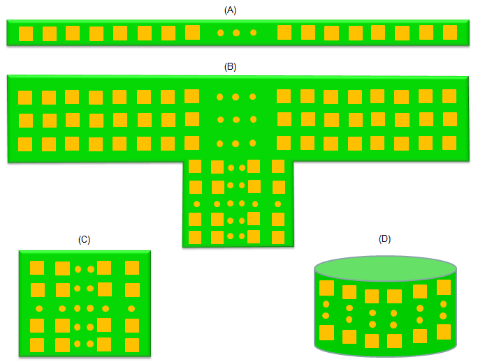
Four Massive MIMO antenna arrangements: a linear row, a wide panel with a vertical extension, a compact rectangular panel, and a cylindrical array

< Figure 1. Four ways to arrange the same set of antenna elements. (A) steers in one plane, and (B), (C) and (D) steer in two. >

(A) is a linear array : One long row of elements steers the beam in azimuth only, and the elevation pattern stays fixed.
(B) is a wide panel with a vertical extension : The three long rows give the horizontal resolution, and the extra block below the centre adds elevation control.
(C) is a compact rectangular panel : The two dimensions are close in size, so the azimuth and elevation resolution are close as well.
(D) wraps the elements around a cylinder : Each part of the surface points a different way, so one unit can cover the full circle.
The dots stand for omitted elements : Every block in the drawing continues, so the element counts drawn are not the counts intended.

How to model the 3D Channel ?

If you arrange the antenna as (B), (C), (D), you would point the direction of the beam both in horizontal and in vertical direction. If you combine the two direction, you can point the beam to any direction in 3D space (at least almost of half of 3D sphere). It is good, but there is complication as well. Now you need to consider the channel factors in all of those direction and you would need mathematical models to take those 3D factors into account.

This kind of channel models are one of the area that require a lot of further study.

How to apply it for FDD Operation ?

I think this is the biggest drawback of Massive MIMO (at least as of now). In order to perform the best beamforming, you need to have accurate (detailed) information of channels that is continuously changing. In order to get this kind of information, you need to get the report from UE on downlink channel quality. To do this, you need to allocate a lot of resources for downlink reference signal which would cause serious waste of resource. In FDD, we don't have any good idea to get the channel information without using this kind of channel quality report based on reference signal.

However in TDD, we can use some alternative technology which may not require this kind of UE reporting. In TDD, we are using the same frequency band for both downlink and uplink. So if Network can estimate the uplink channel quality from UE transmission signal, you can use that information as downlink channel quality. Therefore, in TDD you can create pretty optimized beam without getting explicit channel quality report from UE.

Of course, the estimation derived from uplink signal may not be exactly same as downlink signal because timeslot for uplink and downlink is different. So the channel estimation for UL at a certain timeslot may not be exactly same as the downlink slot. However, this is the most commonly accepted and practiced idea as of now.

Due to this reason, most of Massive MIMO implementation are being done in TDD mode.

How to reduce the amount of Channel Feedback ?

The FDD question above has a second half, and TDD does not remove it. Reciprocity gives the base station the spatial channel. It does not tell the base station how much interference the UE actually sees. So a report still travels upward in either duplex mode, and the size of that report is the problem.

The size grows with the number of ports. NR caps CSI-RS at 32 ports, and that cap bounds what the UE has to measure and what it has to send back. The report itself is written as an index into a codebook that both sides already hold.

NR defines more than one codebook family, and they differ in how much detail they carry. Type I reports a single beam index, so it is small and coarse. Type II reports a weighted combination of beams, with an amplitude and a phase for each one. Type II is the family MU-MIMO needs, because nulling the interference between two users needs detail that a single beam index does not carry.

That detail has a direct cost. A Type II report can be an order of magnitude larger than a Type I report on the same panel. Enhanced Type II in Rel-16 compresses it in the frequency domain, and the Rel-17 port selection codebook compresses it further. Both of them reduce the report. Neither of them removes the growth with port count.

Two directions are being studied from here. The first keeps the codebook and makes the compression smarter. The second replaces the codebook with a learned encoder in the UE and a matching decoder in the gNB. CSI feedback compression was one of the three use cases in the Rel-18 study on AI/ML for the air interface, and the work continued into Rel-19.

The learned option carries a problem the codebook option does not have. The encoder and the decoder are one model split across two vendors. Both halves have to be trained together, and both have to be updated together. How to specify that pairing, and how to test it in a laboratory, is still open.

So the overhead question has become two questions. The first is how small the report can be made. The second is how much of a trained model a specification is willing to carry.

The report grows with the port count : NR caps CSI-RS at 32 ports, which bounds the measurement and the feedback at the same time.
Type II is large because it is detailed : MU-MIMO needs that detail to null the interference between two users, and a beam index does not carry it.
Codebook compression reduces the size, not the trend : Enhanced Type II and the port selection codebook shrink the report, and the growth with ports remains.
A learned encoder is a two vendor model : The UE side and the network side have to be trained and updated together, and that pairing is the open part.

How to generate wide beam from a large array ?

One of the key idea behind Massive MIMO is to increase Antenna gain by constructively adding up multiple antenna output to a single beam and by this process the width of the resulting beam tends to get narrower. We can say this narrow beam is good in terms of energy density, but it also means the area covered by a beam would be very narrow. It means that the beamforming and directing should be very quick and accurate to properly focus on the target UE, but this is not always simple and easy especially when the UE is in fast moving condition.

So it would be necessary to widen the beam width without sacrificing too much of the performance of the massive MIMO.

The place this becomes a hard requirement is initial access. A narrow beam can only serve a UE the network has already found. SSB, SIB1 and paging have to reach a UE whose position is not yet known. So the broadcast channels need a beam wide enough to cover the sector, while the data channels want the narrowest beam the array can make.

The physics works against that. For a uniform linear array with half wavelength spacing, the half power beamwidth is roughly 102 degrees divided by the number of elements. A row of 32 elements therefore gives about 3 degrees. A sector needs about 120 degrees. That is the gap this problem has to close.

Three ways of closing it fit in one drawing. Two of them change what the array does in space. The third keeps the narrow beam and moves the problem into time.

< Figure 2. Three ways to cover a sector. The aperture is the same in all three, and only the excitation across it changes. >

The first method turns elements off. A shorter aperture gives a wider beam, and the array gain falls by the same factor that the aperture lost. It is the simplest method, and it leaves most of the array unused.

The second method keeps every element transmitting and spoils the phase across the aperture. A quadratic or pseudo random phase profile widens the main lobe on purpose. Every amplifier still runs at its full output, so the total radiated power is preserved. That is why phase spoiling is preferred over switching elements off.

The third method keeps the narrow beam and sweeps it. NR does this for SSB, with up to 64 beams inside one 5 ms half-frame in FR2. Coverage is then bought in time rather than in beam width. The cost is the sweep overhead, and the delay a UE waits until its own beam is transmitted.

Two questions stay open. There is no agreed optimum phase profile for a very large array. The choice also interacts with the amplifier design, because a spoiled beam changes the peak to average ratio each amplifier sees. The second question belongs to deployment. A wide SSB beam and a narrow data beam do not reach the same distance. So the cell edge measured on SSB is not the cell edge the data channel can serve.

The broadcast channels set the requirement : SSB, SIB1 and paging have to reach a UE whose position the network does not yet know.
Beamwidth follows the aperture : About 102 degrees divided by the element count, so 32 elements in a row give about 3 degrees.
Phase spoiling keeps the power : Switching elements off loses their gain, while a spoiled phase keeps every amplifier transmitting.
Sweeping buys coverage in time : NR transmits up to 64 SSB beams in one 5 ms half-frame, and the cost appears as overhead and delay.
The broadcast beam and the data beam differ in reach : A cell edge measured on SSB is not the cell edge the data channel can serve.

How to Calibrate the Antenna System ?

Anybody who has experience of RF/mmWave design or testing would understand that the complexity and difficulties of design/testing would increase exponentially as you have more signal path. Even assuming that the design is properly done, you have to make it sure that all of the signal path and antenna are properly calibrated in order for the antenna system to work as intended. Calibrating those huge number of antenna path is definitely challenging task.

Calibration has an exact meaning for an array. A beam exists only as a relative phase and amplitude between the paths. An unknown extra delay on one path rotates that element's contribution against the others. The precoder then points the beam somewhere other than where it computed.

The sensitivity can be stated as a number. Random phase errors across the elements reduce the array gain by roughly the exponential of minus the error variance. A standard deviation of 20 degrees costs about 0.5 dB. Larger errors cost more gain, and they also raise the sidelobes. The sidelobes are the part that matters for MU-MIMO, because a raised sidelobe is interference for another user.

The measurement itself runs inside the unit, and it answers a question that the air interface cannot answer on its own.

< Figure 3. The calibration path, and the limit of reciprocity. The coupler network exists because the reciprocity of the propagation channel says nothing about the chains behind the antennas. >

Figure 3 shows the internal path on the left. A coupler on each transmit path samples a known signal, a combining network brings those samples to one shared receiver, and each path is then compared against a reference path. Transmit calibration and receive calibration are separate procedures, because they measure different hardware.

The right side of Figure 3 is the part that connects this section to the FDD discussion above. In TDD the propagation channel between the two antennas is reciprocal. The transmit chain and the receive chain are not reciprocal, because they are different hardware with different delays. So an uplink measurement predicts the downlink only after the two chains have been calibrated against each other. Reciprocity based beamforming therefore depends on calibration, and not only on the duplex mode.

Calibration is also not a factory step alone. Amplifiers, filters and converters drift with temperature and with age. So the procedure has to run while the base station is carrying traffic, in gaps that the scheduler has to leave for it.

Two things stay open for very large arrays. The coupler network grows with the array, until the calibration hardware approaches the complexity of the array it measures. It is also still argued how much of this can be done over the air, using UE measurements or a neighbouring array, instead of a dedicated internal network.

A beam is a set of relative phases : An unknown delay on one path moves the beam away from the direction the precoder computed.
The gain loss can be quantified : Random phase errors with a standard deviation of 20 degrees cost about 0.5 dB of array gain.
Reciprocity covers the air and not the chains : The transmit chain and the receive chain are different hardware, so TDD beamforming still needs them calibrated against each other.
Drift makes it a runtime procedure : Temperature and ageing move the paths, so calibration runs in service and needs gaps from the scheduler.
The calibration network scales with the array : On a very large array the measuring hardware approaches the complexity of the array itself.

How to handle the complexity of Scheduling and Precoding ?

As you know, the biggest motivation of the Massive MIMO is to increase the directivity and gain for specified target devices. Another motivation (or requirement caused by beam forming) is to implement MU-MIMO (Multi-User MIMO). However, the scheduling and Precoding would get more complicated as more antenna is used and more user is targetted. How to handle this kind of situation would be a big question. Just to increase DSP power ? or to come up with a new/smart mathematical method to handle this without increasing DSP requirement too much ?

The size of the problem is easier to see with numbers. A MU-MIMO scheduler picks a subset of users to share one resource. Choosing 4 users out of 20 candidates gives 4845 possible groups. That choice repeats for every resource block group, and it repeats every slot. At 30 kHz subcarrier spacing a slot lasts 500 microseconds.

The precoder is the second cost. Zero forcing needs the Gram matrix of the channel, and then the inverse of it. Forming the Gram matrix grows with the square of the user count times the port count. The inverse grows with the cube of the user count. So more ports make the first term expensive, and more paired users make the second term expensive.

The two problems are also coupled, and that is what makes the exact solution unreachable. The best set of users depends on the precoder gain each set would achieve. The precoder in turn depends on which set was chosen. Solving both together is the correct formulation, and no real base station solves it that way.

What is done instead is greedy. The scheduler adds users one at a time, and at each step it takes the user whose channel is most orthogonal to the users already selected. That needs a number of passes proportional to the candidate count, rather than a visit to every subset. Regularised zero forcing then replaces the exact inverse, because it behaves better when two paired channels are nearly parallel.

One more limit applies to everything above, and it caps how much computation is worth spending. The channel used by the precoder was measured in an earlier slot. At 3.5 GHz and 120 km/h the coherence time is near 1 millisecond, which is about two slots at 30 kHz spacing. A precoder computed to more precision than the channel will keep is precision spent for nothing.

So the question this section opened with has a sharper form. It is not only whether to add DSP power or to find better mathematics. It is how much of the optimum can be sacrificed for a decision that must finish inside one slot, and still be correct at the moment it is transmitted.

The user selection is combinatorial : Choosing 4 users from 20 gives 4845 groups, and the choice repeats per resource block group and per slot.
The precoder cost splits in two : The Gram matrix grows with the square of the user count times the port count. The inverse grows with the cube of the user count.
Scheduling and precoding are coupled : The best user set depends on the precoder, and the precoder depends on the user set.
Greedy selection is what runs in practice : Users are added one at a time by channel orthogonality, and regularised zero forcing replaces the exact inverse.
Channel aging caps the useful precision : At 3.5 GHz and 120 km/h the coherence time is near 1 ms, which is about two slots at 30 kHz spacing.

How to keep the Power Consumption and Cost under control ?

An antenna element is cheap. What sits behind each element is not, and Figure 1 hides all of it. Each arrangement drawn there assumes the electronics behind the panel already exist. So the real question is not how many elements to build. It is how many of them get a transmit and receive chain of their own.

A fully digital array gives one transmit and receive chain per element. Each chain carries a converter, a mixer, a filter and a power amplifier. With 256 elements that is 256 chains, so the cost and the power follow the element count directly.

The converter is the part that scales worst. The power an ADC needs grows with the sampling rate, and it grows faster still with the number of resolution bits. A wide mmWave carrier needs a high sampling rate. So a fully digital array at those bandwidths becomes expensive in power before it becomes expensive in parts.

The accepted answer today is hybrid beamforming, and there are three architectures worth putting side by side.

< Figure 4. Three array architectures. Each transceiver unit removed lowers the cost and the power, and it also removes one layer of spatial multiplexing. >

Figure 4 puts the three arrangements in one drawing. A fully digital array steers every element on its own. A hybrid array uses analog phase shifters to group several elements into one subarray, and each subarray connects to a single transceiver unit. An analog array is the extreme case, with one transceiver unit for the whole panel.

Hybrid buys the cost reduction with a hard limit. The number of layers a base station can transmit at once cannot exceed the number of transceiver units. A panel with 256 elements and 32 transceiver units therefore has 256 elements worth of array gain and 32 chains worth of multiplexing.

The power amplifier is a second cost, and it is a running one. OFDM has a high peak to average power ratio, so each amplifier has to be operated below its saturation point. That back-off lowers the efficiency, and a few hundred amplifiers at low efficiency become heat inside a sealed unit on a mast.

One direction under study keeps the fully digital array and lowers the converter resolution instead. One to three bits per sample makes a chain per element affordable again. The quantisation noise then has to be carried through the detector, and the detector design is where the difficulty now appears.

So the architecture is a choice among three things. The cost, the number of simultaneous layers, and the freedom to point every element independently. No single point on that curve has become the standard answer.

Elements are cheap and chains are not : The cost and the power follow the number of transceiver units, not the number of radiating elements.
Hybrid beamforming caps the layer count : A panel can transmit no more simultaneous layers than it has transceiver units.
Amplifier back-off is a running cost : The peaks of an OFDM waveform force each amplifier away from saturation, and the lost efficiency appears as heat.
Low resolution converters are the other direction : One to three bits per sample keeps a chain per element, and moves the difficulty into the detector.

How to handle the Near Field of a large Array ?

Every beamforming equation on this page starts from one assumption. The wave arriving at the array is flat across the whole aperture. That assumption is safe for a small antenna. A large aperture is exactly the case where it stops being safe.

The boundary has a name and a formula. The Rayleigh distance is 2D² / λ, where D is the largest dimension of the array. Beyond that distance the wavefront is flat enough to treat as a plane wave. Inside it the wavefront is measurably curved.

The two regimes are easier to see side by side than to derive.

< Figure 5. The same array seen from two distances. Inside the Rayleigh distance the phase across the aperture carries range information, and outside it carries angle alone. >

Two numbers show where that boundary actually falls. A 32 by 32 panel at 28 GHz has a diagonal near 0.24 m, and the Rayleigh distance is then about 10 m. An aperture of 0.5 m at the same frequency pushes it to about 47 m. The first number covers only the space directly in front of the panel. The second covers a part of the cell that carries real users.

Inside that distance the phase across the array depends on the range to the user as well as the angle. A steering vector built from the angle alone no longer aligns every element. So the array loses part of the gain it was built for.

The same effect also has a benefit. A curved wavefront can be focused on a point, rather than steered along a direction. Two users at the same angle and at different ranges then become separable. A far field array cannot separate that pair at all.

Two parts of the specification assume the far field today. The codebooks describe a beam by its angle and carry no distance term. The channel model in TR 38.901 places the scatterers under a plane wave assumption at the array. Both would need a range dimension before near field operation could be configured.

This is mostly a 6G topic, and the extremely large aperture array is where it is being studied. It already appears at mmWave whenever the aperture is large enough.

The Rayleigh distance sets the boundary : 2D² / λ grows with the square of the aperture, so a larger array pushes the near field further out.
A far field steering vector loses gain inside it : Angle alone no longer aligns every element when the wavefront across the aperture is curved.
Curvature also carries range : Beam focusing can separate two users sitting at the same angle and at different distances.
The present codebooks have no distance term : A beam is described by its angle only, so near field operation cannot be configured today.

How to Test and Measure such a System ?

The calibration section above assumes one thing that is easy to miss. Somebody can measure what each path is doing. On an integrated mmWave array, nobody can. The measurement problem then moves outside the unit, and it becomes a question about chambers, distances and test time. Every requirement in this section is shaped by that one missing connector.

An active antenna system puts the radio and the antenna in one sealed unit. There is no connector between the amplifier and the radiating element, so there is no conducted test port. Every radio requirement therefore has to be defined over the air.

That is why the NR base station requirements in TS 38.104 exist in a radiated form. Conducted output power becomes EIRP (Equivalent Isotropic Radiated Power), and conducted sensitivity becomes a sensitivity defined for a direction. The requirement now belongs to a direction in space, rather than to a connector on a panel.

Measuring over the air makes the far field distance a test problem again. A true far field measurement of a 0.5 m aperture at 28 GHz needs a chamber tens of metres long. A compact antenna test range uses a shaped reflector to form a plane wave within a few metres instead. A near field scan with a transform to the far field is the other common method.

Test time is the harder cost. A radiated measurement is taken beam by beam, direction by direction, and band by band. An array with hundreds of beams multiplies every sweep by the beam count. A production line cannot pay for a full sphere per unit.

So the open question is not how to measure one beam. It is how few measurements are enough to declare a whole array good, and how to keep that sample valid as the unit ages in the field.

An integrated array has no test port : The amplifier and the radiating element share one sealed unit, so conducted measurement is not available.
The requirements move to a radiated form : EIRP replaces conducted power in TS 38.104, and the sensitivity is defined for a direction.
The far field distance becomes a chamber size : A compact antenna test range or a near field transform replaces a chamber tens of metres long.
Test time scales with the beam count : A full sphere per beam is affordable in a laboratory and not on a production line.