In this note, we explore a comprehensive Python-based implementation for detecting and decoding the Physical Broadcast Channel (PBCH) from a 5G NR downlink signal using py3gpp and a SigMF-compliant dataset. The script walks through the entire PBCH decoding pipeline—from loading and preprocessing the raw IQ samples to identifying SSBs, estimating and compensating channel effects, and finally performing polar decoding of the broadcasted system information. Leveraging 3GPP-compliant signal processing functions through the py3gpp library, this analysis not only demonstrates signal acquisition and demodulation techniques, but also provides deep insights into equalization, noise handling, and decoding performance in realistic radio environments.
- File Loading and Preprocessing
- Spectrum overview and SSB detection
- SSB Resource Grid
- Channel Estimation and Equalization
- PBCH Decoding
File Loading and Preprocessing
The first stage of the pipeline focuses on loading the downlink signal and preparing it for further processing.
|
#The code begins by reading a SigMF-compliant IQ recording using the following line. This command loads the .sigmf-data file containing the raw complex baseband samples handle = sigmf.sigmffile.fromfile('30720KSPS_dl_signal.sigmf-data')
# Following this, some initial parameters are defined: These variables allow for configuring the frequency offset (delta_f) and numerology (mu) of the received waveform. delta_f = 0 f = 1 mu = 0 apply_fine_CFO = 0
# First generate reference sequences This block doesn't generate all possible reference sequences at once. It creates initial, placeholder versions using default IDs (like NID2=0, NcellID=0). These are used to set up the variables, define their type, and perform initial normalization. The actual detection loops later in the code generate the correct reference sequences on-the-fly (e.g., nrPSS(current_NID2) within the NID2 detection loop) to perform correlations and find the true cell parameters. The initially generated pssRef, sssRef, and dmrsRef (after normalization) are primarily used later in the script for plotting the "Expected" points on the constellation diagrams, although ideally, they should be regenerated with the detected NID, NID2, and ibar_SSB before plotting for accuracy. pssRef = nrPSS(0).astype(np.complex128) # Use NID2=0 initially sssRef = nrSSS(0).astype(np.complex128) dmrsRef = nrPBCHDMRS(0, ibar_SSB=0).astype(np.complex128)
# Normalize reference sequences to unit power pssRef = pssRef / np.sqrt(np.mean(np.abs(pssRef)**2)) sssRef = sssRef / np.sqrt(np.mean(np.abs(sssRef)**2)) dmrsRef = dmrsRef / np.sqrt(np.mean(np.abs(dmrsRef)**2))
# Read and preprocess waveform waveform = handle.read_samples() waveform /= max(waveform.real.max(), waveform.imag.max()) # scale max amplitude to 1 fs = handle.get_global_field(sigmf.SigMFFile.SAMPLE_RATE_KEY) waveform = waveform * np.exp(-1j*2*np.pi*delta_f/fs*(np.arange(len(waveform))))
# Normalize waveform to unit power waveform = waveform / np.sqrt(np.mean(np.abs(waveform)**2))
# Add noise with controlled SNR if ADD_NOISE: np.random.seed(NOISE_SEED) # for reproducible noise
# Calculate required noise power for target SNR signal_power = np.mean(np.abs(waveform)**2) noise_power = signal_power / (10**(TARGET_SNR_DB/10)) noise_std = np.sqrt(noise_power/2) # Standard deviation for real and imaginary parts
# Generate complex Gaussian noise noise = (np.random.normal(0, noise_std, waveform.shape[0]) + 1j * np.random.normal(0, noise_std, waveform.shape[0]))
# Add noise to waveform waveform += noise
# Calculate actual SNR actual_snr_db = 10 * np.log10(signal_power / np.mean(np.abs(noise)**2)) print(f'Target SNR = {TARGET_SNR_DB} dB') print(f'Actual SNR = {actual_snr_db:.1f} dB') |
Spectrum overview and SSB detection
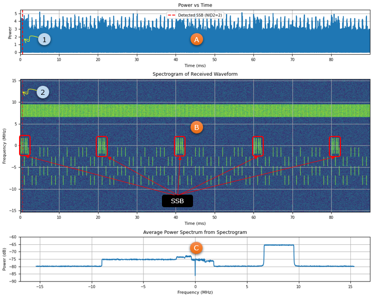
The first step begins with capturing raw IQ samples from a SigMF-formatted downlink recording(a save IQ file), followed by power analysis and SSB detection using correlation with reference waveforms. The visualized output of this step is shown below.
The plot (A) illustrates the time-domain power profile of the received signal, highlighting the moment an SSB burst is detected. The spectrogram (B) offers a detailed time-frequency representation, revealing the periodic structure and spectral occupancy of the waveform. Finally, the plot (C) summarizes the average power spectrum, showing clear frequency bands where signal energy is concentrated. These plots not only validate the integrity of the signal but also provide critical timing and spectral insights necessary for accurate demodulation and decoding of the PBCH. The red line marked as (1) and (2) indicates the position of SSB by the script in this note.
Preprocessor and Basic Calculation
This code block configures the expected signal structure, then generates each of the three possible PSS signals, correlates them against the received waveform, and identifies which PSS sequence gives the strongest correlation peak, thereby detecting NID2. This is a fundamental first step in synchronizing to a 5G cell
|
# Carrier Configuration This block configures the fundamental parameters of the 5G New Radio carrier being analyzed. It uses nrCarrierConfig to set the channel bandwidth via NSizeGrid = 106, indicating 106 Physical Resource Blocks (which commonly corresponds to a 20 MHz bandwidth for the typical 15 kHz subcarrier spacing used in synchronization), and defines the SubcarrierSpacing itself, likely set to 15 kHz based on the numerology parameter mu. Subsequently, nrOFDMInfo is used to calculate essential derived OFDM parameters, such as the appropriate FFT size and cyclic prefix lengths, based on this initial carrier configuration. carrier = nrCarrierConfig(NSizeGrid = 106, SubcarrierSpacing = 15 * 2**mu) info = nrOFDMInfo(carrier) Nfft = info['Nfft'] print(f'Nfft = {Nfft}')
# PSS Preparation and Index Calculation This section prepares for the Primary Synchronization Signal (PSS) detection by initializing storage arrays (peak_value, peak_index) to hold the results of correlation tests for the three possible NID2 values. It also defines key constants like the PSS length (PSS_LEN) and the number of resource elements per block (NRE_PER_PRB). Crucially, it calculates the precise frequency subcarrier indices (pssIndices) where the PSS signal is expected to be located, centered within the configured carrier bandwidth. peak_value = np.zeros(3) peak_index = np.zeros(3, 'int')
PSS_LEN = 128 NRE_PER_PRB = 12 This calculates the specific frequency indices (subcarrier numbers) where the PSS is located within the full carrier resource grid defined by NSizeGrid. In this case it is assumed that the PSS is centered in the frequency domain. The calculation finds the center subcarrier of the 106 PRBs and then selects the 128 indices centered around it. ( pssIndices = np.arange((carrier.NSizeGrid * NRE_PER_PRB // 2 - PSS_LEN // 2), (carrier.NSizeGrid * NRE_PER_PRB // 2 + PSS_LEN // 2 - 1))
#NID2 Detection Loop (Correlation)/PSS Detection This block performs the core NID2 detection by systematically testing each of the three possible NID2 values (0, 1, and 2). Within a loop, it generates a candidate time-domain Primary Synchronization Signal (PSS) waveform corresponding to the NID2 value currently being tested. This involves creating the PSS sequence, placing it on a resource grid, performing OFDM modulation, and removing the cyclic prefix. Then, this candidate PSS waveform is cross-correlated with the received signal. The loop finds and stores the magnitude and timing index of the highest correlation peak obtained for each candidate NID2, preparing for the final decision. for current_NID2 in np.arange(3, dtype='int'): slotGrid = nrResourceGrid(carrier) slotGrid = slotGrid[:, 0] slotGrid[pssIndices] = nrPSS(current_NID2) [refWaveform, info] = nrOFDMModulate(carrier, slotGrid, SampleRate = fs) refWaveform = refWaveform[info['CyclicPrefixLengths'][0]:]; # remove CP
temp = scipy.signal.correlate(waveform[:int(25e-3 * fs)], refWaveform, 'valid') # correlate over 25 ms peak_index[current_NID2] = np.argmax(np.abs(temp)) peak_value[current_NID2] = np.abs(temp[peak_index[current_NID2]]) t_corr = np.arange(temp.shape[0])/fs*1e3 #axs[current_NID2].plot(t_corr, np.abs(temp)) detected_NID2 = np.argmax(peak_value)
Since this part is so important, let me break down the block and look into the detailed meaning
|
Power vs Time - (A)
This subplot shows the signal's magnitude over time, helping identify when energy bursts like the SSB appear. A vertical red dashed line marks the estimated timing of the detected SSB based on the strongest correlation with the PSS sequence.
|
t_power = np.arange(len(waveform))/fs * 1000 # Time in milliseconds power_time = np.abs(waveform) ax0.plot(t_power, power_time) ssb_time = peak_index[detected_NID2]/fs*1e3 # Convert to milliseconds ax0.axvline(x=ssb_time, color='r', linestyle='--', label=f'Detected SSB (NID2={detected_NID2})') |
- power_time = np.abs(waveform) computes the magnitude of the complex waveform.
- t_power represents the time axis in milliseconds.
- ax0.axvline(...) plots the red vertical dashed line to mark the SSB detection time using the peak correlation result: peak_index[detected_NID
Spectrogram of Received Waveform - (B)
This subplot (B) provides a time-frequency view of the received signal using a spectrogram. It reveals periodic SSB bursts and overall spectral activity in the signal. The SSB timing line appears again for reference.
|
nperseg = Nfft f, t, Sxx = scipy.signal.spectrogram(waveform, fs=fs, nperseg=nperseg, noverlap=noverlap, return_onesided=False) f = np.fft.fftshift(f) Sxx = np.fft.fftshift(Sxx, axes=0) spec = ax1.pcolormesh(t*1000, f/1e6, 10*np.log10(np.abs(Sxx)), shading='gouraud', cmap='viridis', vmin=-90, vmax=-60) ax1.axvline(x=ssb_time, color='r', linestyle='--', alpha=0.5) |
- The spectrogram is computed using scipy.signal.spectrogram.
- Frequencies (f) and power values (Sxx) are FFT-shifted to center DC at 0.
- The plotting function ax1.pcolormesh(...) displays the spectrogram in dB scale.
- The red dashed line (ax1.axvline(...)) marks the detected SSB timing, aligned with the time axis.
Average Power Spectrum from Spectrogram - (C)
This bottom subplot shows the average spectral power across time, giving an overall view of signal bandwidth and occupied spectrum.
|
power_spectrum = 10*np.log10(np.mean(np.abs(Sxx), axis=1)) ax2.plot(f/1e6, power_spectrum) |
- np.mean(np.abs(Sxx), axis=1) averages the spectrogram power over time.
- Converted to dB scale and plotted over frequency using ax2.plot(...).
Detected SSB Position Marker - (1),(2)
The red vertical dashed line (axvline) appears in both the Power vs Time and Spectrogram subplots, helping align the temporal position of the detected SSB across both time and time-frequency views. It is calculated as:
|
ssb_time = peak_index[detected_NID2]/fs*1e3 |
- where peak_index[...] comes from this correlation-based detection loop:
|
temp = scipy.signal.correlate(waveform[:int(25e-3 * fs)], refWaveform, 'valid') peak_index[current_NID2] = np.argmax(np.abs(temp)) |
- This step identifies the most likely SSB position by matching PSS sequences and detecting the timing offset.
SSB Resource Grid
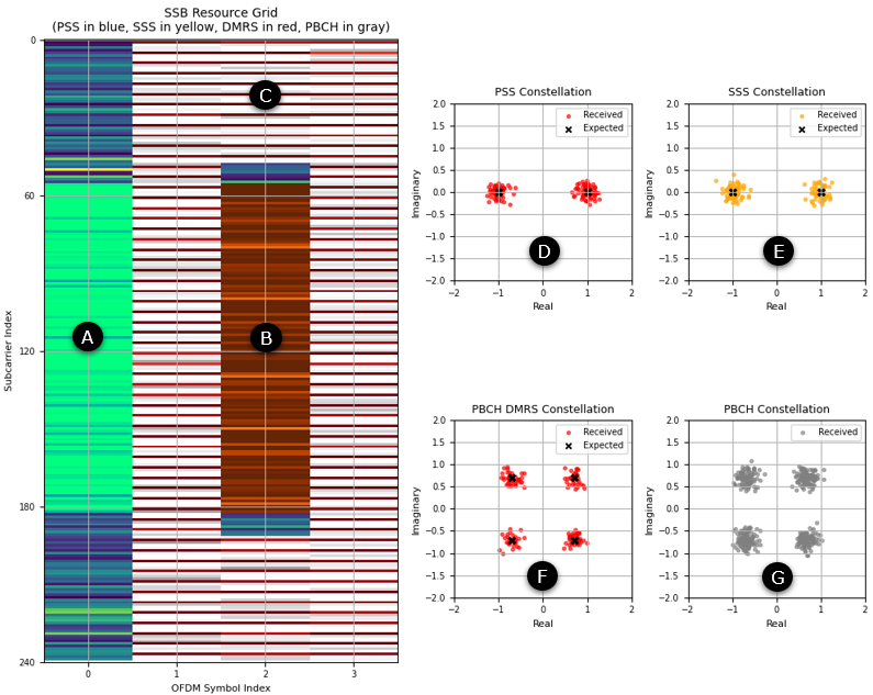
Next step I want to do is to show the grid map of SSB and plot the constellation of each signals and channel in the SSB. The figure shown below presents a detailed view of the 5G NR Synchronization Signal Block (SSB) resource grid, alongside the corresponding constellation diagrams of key downlink signals. The SSB resource grid highlights how individual components—Primary Synchronization Signal (PSS), Secondary Synchronization Signal (SSS), Demodulation Reference Signal (DMRS), and the Physical Broadcast Channel (PBCH)—are mapped in both frequency and time within the OFDM resource grid. The (A),(B),(C) on the resource grid visualizes these allocations, with color-coded overlays indicating the location of each signal type. The accompanying constellation plots provide a snapshot of the received symbols after extraction, enabling visual assessment of signal quality and modulation accuracy. These plots serve as crucial diagnostics for evaluating synchronization performance and physical layer decoding robustness under realistic channel conditions. They collectively provide a complete visual diagnosis of the SSB block, from RE allocation to signal demodulation fidelity, helping verify both synchronization and decoding steps in the 5G NR receiver pipeline.
OFDM Demodulation and Resource Grid Preparation
Before any resource extraction or constellation plotting can happen, the raw time-domain waveform must be converted into its corresponding frequency-domain representation, also known as the resource grid. This is where the physical layer structure of 5G NR (like PSS, SSS, PBCH, DMRS) is spatially laid out in terms of subcarriers and OFDM symbols.
This block takes the received waveform and the previously detected NID2, then performs several crucial steps to further synchronize with the 5G cell and prepare for decoding the broadcast channel. It first refines the timing synchronization, then demodulates the relevant part of the signal into a resource grid. Using this grid, it detects the remaining parts of the physical cell ID (NID1, giving the full NID) and the time index of the Synchronization Signal Block (ibar_SSB). Finally, it identifies and extracts the PSS, SSS, PBCH DMRS, and PBCH data symbols from the demodulated grid.
|
# Basic Parameters for SSB Basic parameters for the SSB are defined: nrbSSB (bandwidth = 20 RBs), scsSSB (subcarrier spacing, likely 15kHz), nSlot (initial slot assumption), and rxSampleRate. nrbSSB = 20 scsSSB = 15 * 2**(mu) nSlot = 0 rxSampleRate = fs
# TimingOffset Estimation This is to find a precise starting point (the timingOffset in samples) within the input waveform that accurately aligns with the beginning of the Synchronization Signal Block (SSB). It does this by utilizing the already detected NID2 to generate the corresponding Primary Synchronization Signal (PSS) and then correlating this known PSS signal against the received waveform to find the point of best match. refGrid = np.zeros((nrbSSB*12, 2), np.complex128) refGrid[nrPSSIndices(), 1] = nrPSS(detected_NID2) timingOffset = nrTimingEstimate(waveform = waveform, nrb = nrbSSB, scs = scsSSB, initialNSlot = nSlot, refGrid = refGrid, SampleRate = rxSampleRate)
Following is the break down of the block
# modulate about 8 symbols, only has to be at least 5 This block first takes the time-synchronized input signal (waveform starting at timingOffset) and converts a portion of it, guaranteed to contain the Synchronization Signal Block (SSB), from the time domain into its frequency domain representation (a resource grid). It then precisely extracts the specific 4 OFDM symbols that make up the SSB from this grid, preparing them for further analysis like signal extraction and decoding. rxGrid = nrOFDMDemodulate(waveform = waveform[timingOffset:][:np.min((len(waveform), 2048*8))], nrb = nrbSSB, scs = scsSSB, initialNSlot = nSlot, SampleRate=rxSampleRate, CyclicPrefixFraction=0.5) rxGrid = rxGrid[:,1:5]
Following is the breakdown of the code
# Normalize by FFT size and additional factor to get correct constellation scaling This line scales the amplitude of all the complex values within the demodulated rxGrid. The main goal is to adjust the overall power level so that the received signal constellation points (PSS, SSS, DMRS, PBCH) align correctly with their expected standard positions, typically having magnitudes around 1, which simplifies visualization and subsequent processing steps like channel estimation or symbol demodulation. rxGrid = rxGrid / (np.sqrt(Nfft) * 3.0) # Factor of 3 to match expected constellation points
# Get SSS indices and convert to frequency indices This block focuses on isolating the Secondary Synchronization Signal (SSS) from the demodulated SSB resource grid (rxGrid). It first identifies the specific resource elements where the SSS is located, extracts the corresponding received complex symbols, and then applies a specific normalization to these symbols, likely to prepare them for the correlation process used to detect NID1. sssIndices = nrSSSIndices() sssRx = nrExtractResources(sssIndices, rxGrid) sssRx /= np.max((sssRx.real.max(), sssRx.imag.max())) # scale sssRx symbols individually
# SSS correlation for NID1 detection This section identifies the remaining component (NID1) needed to determine the full Physical Cell ID (NcellID) of the 5G cell. It achieves this by comparing the received Secondary Synchronization Signal (SSS) symbols, extracted previously (sssRx), against every possible reference SSS sequence. The reference sequence that best matches the received SSS reveals the correct NID1, which is then combined with the already known NID2 to get the full NcellID. sssEst = np.zeros(336) for NID1 in range(335): ncellid = (3*NID1) + detected_NID2 sssRef = nrSSS(ncellid) sssEst[NID1] = np.abs(np.vdot(sssRx, sssRef))
detected_NID1 = np.argmax(sssEst) detected_NID = detected_NID1*3 + detected_NID2
# DMRS correlation for ibar_SSB detection This section determines the specific time index (ibar_SSB) of the received Synchronization Signal Block (SSB) relative to other potential SSBs within a burst. It works by comparing the received Demodulation Reference Signal (DMRS) symbols associated with the Physical Broadcast Channel (PBCH) against reference DMRS sequences generated for different possible ibar_SSB values. The ibar_SSB value whose reference DMRS best matches the received DMRS reveals the index of the received SSB, which is essential information for later PBCH decoding steps (specifically descrambling). dmrsIndices = nrPBCHDMRSIndices(detected_NID, style='matlab') xcorrPBCHDMRS = np.empty(7) for ibar_SSB in range(7): PBCHDMRS = nrPBCHDMRS(detected_NID, ibar_SSB) xcorrPBCHDMRS[ibar_SSB] = np.abs(np.vdot(nrExtractResources(dmrsIndices, rxGrid), PBCHDMRS)) ibar_SSB = np.argmax(np.abs(xcorrPBCHDMRS))
Following is the breakdown of the code and description
# Create masks for PSS and SSS This section initializes several boolean arrays (masks) that have the same dimensions as the rxGrid (which holds the 4 symbols of the SSB). These masks (pss_mask, sss_mask, dmrs_mask, pbch_mask) act like templates, initially all set to False. They will be used in the following steps to mark the specific locations (resource elements) within the rxGrid where each type of signal (PSS, SSS, DMRS, PBCH) resides. pss_mask = np.zeros_like(rxGrid, dtype=bool) sss_mask = np.zeros_like(rxGrid, dtype=bool) dmrs_mask = np.zeros_like(rxGrid, dtype=bool) pbch_mask = np.zeros_like(rxGrid, dtype=bool)
Following is the breakdown of the code and description
# Get PSS indices for SSB grid This block determines the exact frequency locations (subcarrier indices) occupied by the Primary Synchronization Signal (PSS) within the SSB's bandwidth. It then updates the pss_mask (created in the previous step) by marking these specific frequency locations within the first symbol of the SSB grid as True. pssIndices = nrPSSIndices() pss_freq_indices = pssIndices % (nrbSSB * 12) # Convert to frequency indices for SSB grid pss_mask[pss_freq_indices, 0] = True # PSS is in first symbol
Following is the breakdown of the code and description
# Get SSS indices for SSB grid Similar to the PSS masking, this code block determines the specific frequency locations (subcarrier indices) used by the Secondary Synchronization Signal (SSS) within the SSB's bandwidth. It then updates the sss_mask by marking these frequency locations within the third symbol (index 2) of the SSB grid as True. sss_freq_indices = sssIndices % (nrbSSB * 12) # Convert to frequency indices for SSB grid sss_mask[sss_freq_indices, 2] = True # SSS is in third symbol (index 2)
Following is the breakdown of the code and description
# Get PBCH DMRS indices This block identifies the precise time-frequency locations (resource elements) within the 4-symbol SSB grid (rxGrid) where the PBCH DMRS is transmitted. It calculates the specific subcarrier and OFDM symbol indices for every DMRS symbol based on the detected Physical Cell ID (detected_NID) and then marks these locations as True in the dmrs_mask. dmrsIndices = nrPBCHDMRSIndices(detected_NID, style='matlab') symbol_size = nrbSSB * 12 symbol_indices = dmrsIndices // symbol_size # Get symbol indices freq_indices = dmrsIndices % symbol_size # Get frequency indices for i in range(len(freq_indices)): dmrs_mask[freq_indices[i], symbol_indices[i]] = True
Following is the breakdown of the code and description
# Get PBCH indices This code identifies all the potential time-frequency locations (resource elements) within the 4-symbol SSB grid (rxGrid) that are designated for carrying the actual Physical Broadcast Channel (PBCH) data. It calculates the specific subcarrier and OFDM symbol index for each of these potential PBCH locations based on the detected Physical Cell ID (detected_NID) and marks these positions as True in the pbch_mask. Note that this initial marking includes resource elements that are also used for DMRS. pbchIndices = nrPBCHIndices(detected_NID) pbch_symbol_indices = pbchIndices // symbol_size pbch_freq_indices = pbchIndices % symbol_size for i in range(len(pbch_freq_indices)): pbch_mask[pbch_freq_indices[i], pbch_symbol_indices[i]] = True
Following is the breakdown of the code and description
# Remove DMRS positions from PBCH mask to avoid overlap This line performs a logical operation to refine the pbch_mask. Its purpose is to ensure that the final pbch_mask only identifies the resource elements carrying actual PBCH data, by explicitly removing any locations that are occupied by the PBCH DMRS. pbch_mask = pbch_mask & ~dmrs_mask
Following is the breakdown of the code and description
# Extract received signals This block extracts the actual received complex symbols for the Primary Synchronization Signal (PSS), Secondary Synchronization Signal (SSS), and the PBCH Demodulation Reference Signal (DMRS) from the main rxGrid. It uses the specific frequency and symbol indices determined in previous steps to pinpoint these signals within the 4-symbol SSB grid structure. The resulting arrays (pssRx, sssRx, dmrsRx) contain the demodulated values for each respective signal. pssRx = rxGrid[pss_freq_indices, 0] sssRx = rxGrid[sss_freq_indices, 2] dmrsRx = rxGrid[freq_indices, symbol_indices]
Following is the breakdown of the code and description
# Extract PBCH signals (excluding DMRS positions) This block carefully extracts the received complex symbols that correspond only to the actual Physical Broadcast Channel (PBCH) data, explicitly excluding the symbols used for the PBCH DMRS (Demodulation Reference Signal). It achieves this by iterating through the list of all potential PBCH resource element locations but only selecting those that are marked as True in the refined pbch_mask (where DMRS locations have already been set to False). The complex symbols from these validated PBCH data locations are then gathered from the rxGrid into the pbchRx array. pbch_freq_indices_no_dmrs = [] pbch_symbol_indices_no_dmrs = [] for i in range(len(pbch_freq_indices)): if pbch_mask[pbch_freq_indices[i], pbch_symbol_indices[i]]: # Only include if not overlapping with DMRS pbch_freq_indices_no_dmrs.append(pbch_freq_indices[i]) pbch_symbol_indices_no_dmrs.append(pbch_symbol_indices[i]) pbchRx = rxGrid[pbch_freq_indices_no_dmrs, pbch_symbol_indices_no_dmrs]
Following is the breakdown of the code and description
|
This block performs OFDM demodulation on a portion of the received time-domain signal (waveform). It essentially transforms the signal from the time domain back into the frequency domain, organizing it into a resource grid (rxGrid) where each element represents the complex value on a specific subcarrier during a specific OFDM symbol. This step is necessary to access the synchronization signals (like PSS, SSS) and the broadcast channel (PBCH) which are transmitted on specific resource elements within this grid structure.
|
rxGrid = nrOFDMDemodulate( waveform = waveform[timingOffset:][:np.min((len(waveform), 2048*8))], nrb = nrbSSB, scs = scsSSB, initialNSlot = nSlot, SampleRate = rxSampleRate, CyclicPrefixFraction = 0.5 ) |
- rxGrid = nrOFDMDemodulate(...): This function call executes the OFDM demodulation process.
- waveform = waveform[timingOffset:][:np.min((len(waveform), 2048*8))]: This selects the specific segment of the input time-domain waveform to be demodulated.
- waveform[timingOffset:]: It starts processing the waveform from the timingOffset, which was likely calculated previously (e.g., via PSS correlation) to align with the beginning of the Synchronization Signal Block (SSB).
- [:np.min((len(waveform), 2048*8))]: It takes a limited number of samples from the offset point – enough to cover approximately 8 OFDM symbols (assuming an FFT size Nfft=2048, common for a 20 MHz channel), but not exceeding the remaining length of the waveform. This duration is sufficient to contain the 4 symbols of the SSB.
- nrb = nrbSSB: Specifies the bandwidth for demodulation in terms of the number of resource blocks. nrbSSB is typically 20, corresponding to the standard bandwidth of an SSB.
- scs = scsSSB: Defines the subcarrier spacing (e.g., 15 kHz or 30 kHz) associated with the SSB being demodulated.
- initialNSlot = nSlot: Indicates the starting slot number context for the demodulation.
- SampleRate = rxSampleRate: Provides the sample rate of the input waveform, which is essential for the demodulator's internal calculations (like FFT windowing and symbol timing).
- CyclicPrefixFraction = 0.5: This parameter likely relates to how the function handles the removal of the cyclic prefix, possibly defining a search window or an assumed fractional starting point for the useful part of the symbol, helping to cope with minor timing errors.
|
rxGrid = rxGrid[:,1:5] |
-
This selects OFDM symbols 1 through 4, which correspond to the active portion of the SSB.
-
SSB elements like PSS, SSS, DMRS, and PBCH all reside in these symbols.
|
rxGrid = rxGrid / (np.sqrt(Nfft) * 3.0) |
-
The grid is normalized by the FFT size to correct for energy scaling.
-
The extra factor of 3.0 is empirically chosen to match the expected constellation amplitude (e.g., QPSK at ±1/√2).
-
Without this, constellation diagrams would appear incorrectly scaled and may affect demodulation accuracy.
SSB Resource Grid - Background Layer
This section visualizes the background layer of the SSB resource grid by plotting the magnitude of received elements that are not part of PSS, SSS, DMRS, or PBCH. It uses the rxGrid, which is the demodulated frequency-domain grid, and applies a viridis colormap to highlight only the non-overlapping resource elements. The np.where condition filters out all known signal positions, allowing the viewer to focus on unused or residual areas within the grid structure.
|
ssb_data = np.abs(rxGrid)
plt.imshow(np.where(~(pss_mask | sss_mask | dmrs_mask | pbch_mask), ssb_data, np.nan), aspect='auto', interpolation='none', cmap='viridis') |
- rxGrid is the demodulated resource grid extracted from the waveform.
- ssb_data contains the magnitudes of the received resource elements.
- The background layer shows all non-occupied (non-PSS, non-SSS, non-DMRS, non-PBCH) REs in the grid using a viridis colormap.
- np.where(...) ensures only non-overlapping REs are shown in this layer.
PBCH Layer in the Grid
This part of the visualization overlays the PBCH (Physical Broadcast Channel) resource elements on the SSB grid using a gray colormap. The pbch_mask identifies where PBCH symbols are located within the grid, and these values are displayed on top of the existing background layer. The corresponding amplitudes from ssb_data are rendered only at the positions marked by the mask, allowing a clear distinction of the PBCH structure within the overall resource allocation.
|
plt.imshow(np.where(pbch_mask, ssb_data, np.nan), aspect='auto', interpolation='none', cmap='gray', vmin=0, vmax=1) |
- This overlay highlights PBCH REs using a gray colormap.
- pbch_mask is a boolean mask identifying the PBCH RE positions.
- These are rendered on top of the background layer with their respective signal amplitudes.
DMRS, PSS, SSS Layers in the Grid
This section overlays the positions of DMRS, PSS, and SSS onto the SSB resource grid using color-coded layers. The DMRS elements are shown in red, PSS in blue (using the 'winter' colormap), and SSS in yellow-orange (using 'YlOrBr'), each identified by their respective boolean masks. These overlays are rendered on top of the background grid, allowing clear visual differentiation of the individual reference signal components. The np.where condition ensures that only the relevant resource elements for each signal type are displayed, effectively isolating their structure within the overall grid.
|
plt.imshow(np.where(dmrs_mask, ssb_data, np.nan), aspect='auto', interpolation='none', cmap='Reds', vmin=0, vmax=1) plt.imshow(np.where(pss_mask, ssb_data, np.nan), aspect='auto', interpolation='none', cmap='winter', vmin=0, vmax=1) plt.imshow(np.where(sss_mask, ssb_data, np.nan), aspect='auto', interpolation='none', cmap='YlOrBr', vmin=0, vmax=1) |
- These lines add overlay layers for each reference signal:
- DMRS in red,
- PSS marked as (A),
- SSS marked as (C)
- The masks (*_mask) define RE positions, and np.where filters out irrelevant points.
PSS Constellation - (D)
This plot visualizes the constellation of the Primary Synchronization Signal (PSS) by comparing the received symbols to the expected reference sequence. The variable pssRx holds the complex-valued received PSS samples extracted from the demodulated resource grid, while pssRef contains the locally generated reference PSS sequence. Using a scatter plot, the received symbols are plotted in red and semi-transparent, while the ideal constellation points are marked in black with 'x' markers. This allows for a direct visual assessment of how accurately the receiver captured the PSS under current channel conditions.
|
plt.scatter(pssRx.real, pssRx.imag, c='red', alpha=0.6, s=30, marker='.', label='Received') plt.scatter(pssRef.real, pssRef.imag, c='black', s=20, marker='x', label='Expected') |
- pssRx contains the received PSS samples extracted from rxGrid.
- pssRef is the locally generated reference sequence.
- This scatter plot compares the received PSS constellation to the ideal one.
SSS Constellation - (E)
This subplot displays the Secondary Synchronization Signal (SSS) constellation, comparing the received and reference symbols. The variable sssRx contains the SSS samples extracted from the demodulated grid, while sssRef holds the ideal SSS sequence generated based on the detected cell ID. The plot uses orange dots to show the received symbols and black 'x' markers to indicate the expected positions. By comparing the two, one can assess how accurately the receiver has captured and demodulated the SSS in the presence of noise and channel distortion.
|
plt.scatter(sssRx.real, sssRx.imag, c='orange', alpha=0.6, s=30, marker='.', label='Received') plt.scatter(sssRef.real, sssRef.imag, c='black', s=20, marker='x', label='Expected') |
- sssRx is the extracted SSS from the grid.
- sssRef is the corresponding reference.
- This plot visualizes how closely the received SSS matches the expected constellation.
PBCH DMRS Constellation - (F)
This plot illustrates the PBCH DMRS (Demodulation Reference Signal) constellation, comparing received symbols to their expected values. The dmrsRx array holds the DMRS samples extracted from the resource grid using predefined DMRS indices, while dmrsRef contains the corresponding ideal sequence generated based on the detected NID and ibar_SSB. The received points are plotted in red, and the reference points are shown in black with 'x' markers. This comparison is crucial for evaluating the quality of the channel and the accuracy of the channel estimation used later during PBCH equalization.
|
plt.scatter(dmrsRx.real, dmrsRx.imag, c='red', alpha=0.6, s=30, marker='.', label='Received') plt.scatter(dmrsRef.real, dmrsRef.imag, c='black', s=20, marker='x', label='Expected') |
- dmrsRx includes the received DMRS samples extracted using the known DMRS indices.
- dmrsRef is generated based on the detected NID and ibar_SSB.
- Comparing these helps assess channel quality and estimation performance
PBCH Constellation - (G)
This constellation plot shows the received PBCH symbols after excluding the DMRS positions. The data points in pbchRx are plotted in gray, representing the raw QPSK-modulated PBCH values as captured from the resource grid. No reference symbols are plotted in this case, since the transmitted PBCH content depends on encoded system information bits, which vary between transmissions. The plot provides a visual impression of modulation quality and potential impairments affecting the PBCH without making assumptions about the encoded data.
|
plt.scatter(pbchRx.real, pbchRx.imag, c='gray', alpha=0.6, s=30, marker='.', label='Received') |
- pbchRx contains the received PBCH samples (excluding DMRS REs).
- Only the received points are plotted here (no reference overlay), since QPSK-modulated PBCH symbols vary depending on the encoded system info bits.
Channel Estimation and Equalization
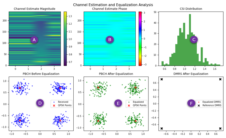
Next step is to perform a detailed visualization of the channel estimation and equalization process applied to the received 5G NR PBCH signal. The top row illustrates key characteristics of the estimated channel: the magnitude and phase distributions across the resource grid, along with a histogram of Channel State Information (CSI) values that reflect signal quality. In the bottom row, constellation diagrams compare PBCH symbols before and after equalization, showing the improvement in symbol clarity and alignment with ideal QPSK positions. The final plot highlights the equalized DMRS symbols against their reference counterparts, serving as a validation of channel correction accuracy. Altogether, this figure offers insight into how well the receiver characterizes and compensates for the wireless channel's impairments to recover transmitted data.
Preprocess and Calculation
|
import matplotlib.patches as mpatches
if not SKIP_EQUALIZATION:
# Create reference grid with matching dimensions These lines prepare a template grid (refGrid) that mirrors the structure of the received SSB signal grid (rxGrid). This template grid will then be populated with the known reference signals (specifically the PBCH DMRS) at their correct locations. This refGrid, containing only the known DMRS pilots, is essential for performing channel estimation in the subsequent steps refGrid = np.zeros((nrbSSB*12, 4), 'complex') dmrsIndices = nrPBCHDMRSIndices(detected_NID, style='matlab')
Followings are the breakdown and description
# Set DMRS reference signals This line takes the known, ideal PBCH DMRS (Demodulation Reference Signal) sequence and places it into the correct time-frequency locations within the refGrid (which was previously initialized as an empty grid of zeros). This step creates a clean reference grid containing only the expected DMRS pilot symbols, which is crucial for comparing against the received grid (rxGrid) to estimate the radio channel conditions. nrSetResources(dmrsIndices, refGrid, nrPBCHDMRS(detected_NID, ibar_SSB))
Followings are the breakdown and description
# Channel estimation using reference implementation method This code performs channel estimation, which is the process of figuring out how the radio channel altered the signal. It does this by comparing the received pilot symbols (DMRS) within rxGrid to the known, ideal DMRS symbols stored in refGrid. By analyzing the differences in amplitude and phase at these known points, the function estimates the channel's effect (represented by H) across the entire time-frequency grid and also estimates the level of noise (nVar) present in the received signal. with np.errstate(divide='ignore', invalid='ignore'): H, nVar = nrChannelEstimate(rxGrid=rxGrid, refGrid=refGrid)
Followings are the breakdown and description
# DMRS equalization This line performs a basic form of channel equalization specifically on the PBCH DMRS (Demodulation Reference Signal) symbols. It attempts to remove the distorting effects of the radio channel from the received DMRS symbols by dividing the received signal (rxGrid) by the estimated channel response (H). The resulting "channel-corrected" DMRS symbols are then extracted and stored. PBCHDMRS_wiped = nrExtractResources(dmrsIndices, rxGrid/H)
Followings are the breakdown and description
# PBCH equalization using MMSE This block performs channel equalization specifically on the symbols intended for the Physical Broadcast Channel (PBCH) data, using the Minimum Mean Square Error (MMSE) technique. Unlike simple zero-forcing, MMSE equalization considers both the estimated channel effect (H) and the estimated noise level (nVar) to calculate an equalization filter that optimally reverses the channel distortion while minimizing noise amplification. The outputs are the equalized PBCH symbols (pbch_eqed) ready for demodulation, and Channel State Information (csi) values indicating the quality/reliability of the channel at those locations. pbchIndices = nrPBCHIndices(detected_NID) pbch_eqed, csi = nrEqualizeMMSE(nrExtractResources(pbchIndices, rxGrid), nrExtractResources(pbchIndices, H), nVar)
Followings are the breakdown and description
# Calculate EVM This line calculates the Error Vector Magnitude (EVM) for the equalized PBCH data symbols (pbch_eqed). EVM is a standard metric used to quantify the quality of a digitally modulated signal by measuring the difference between the actual received constellation points (after equalization) and their ideal target locations. A lower EVM value indicates a cleaner signal with less distortion and noise. evm = np.sum(np.abs(pbch_eqed - nrSymbolModulate(nrSymbolDemodulate(pbch_eqed, 'QPSK', 1, 'hard'), 'QPSK'))) / pbch_eqed.shape[0]
Followings are the breakdown and description
|
Channel Estimate Magnitude - (A)
This plot visualizes the magnitude of the estimated channel matrix, providing insight into how much gain or attenuation each resource element experienced as the signal propagated through the wireless channel. The channel matrix H is computed using the nrChannelEstimate function, which compares the received grid against known reference signals. Taking the absolute value of H reveals the signal strength variations across the time-frequency grid, and the result is rendered using a color map to highlight areas of strong and weak reception. This helps assess the reliability of different regions in the SSB grid.
|
ax_ch_mag = fig_eq.add_subplot(eq_grid[0, 0]) ch_mag_plot = ax_ch_mag.imshow(np.abs(H), origin='lower', aspect='auto', cmap='viridis') |
- H is the estimated channel matrix computed using:
- H, nVar = nrChannelEstimate(rxGrid=rxGrid, refGrid=refGrid)
- np.abs(H) gives the magnitude of each complex channel estimate.
- This plot shows how much gain each resource element experienced through the channel.
Channel Estimate Phase - (B)
This plot displays the phase component of the estimated channel matrix, offering a view into how the signal’s phase has been altered during transmission. The phase is extracted from the complex channel estimate H using np.angle(H), and is visualized using an HSV colormap to represent the full range from −π to π. Variations in phase across the grid can reveal frequency offsets, Doppler shifts, or multipath effects that cause distortion in the received signal. This visualization is critical for understanding the non-amplitude-related impairments introduced by the wireless channel.
|
ax_ch_phase = fig_eq.add_subplot(eq_grid[0, 1]) ch_phase_plot = ax_ch_phase.imshow(np.angle(H), origin='lower', aspect='auto', cmap='hsv', vmin=-np.pi, vmax=np.pi) |
- np.angle(H) extracts the phase of each channel estimate.
- The HSV colormap helps visualize the phase spectrum between −π and π
- Phase distortion can indicate the presence of frequency offset or multipath effects.
CSI Distribution (Channel State Information) - (C)
This histogram visualizes the distribution of Channel State Information (CSI) values obtained during the MMSE equalization process. CSI reflects the reliability or confidence of each equalized PBCH symbol and is computed alongside the equalized signal using the nrEqualizeMMSE function. By plotting the frequency of CSI values across all PBCH resource elements, this chart provides a statistical view of how well the channel was estimated and how trustworthy each demodulated bit is likely to be under current conditions.
|
ax_csi = fig_eq.add_subplot(eq_grid[0, 2]) ax_csi.hist(csi, bins=30, color='green', alpha=0.7) |
- csi is computed during MMSE equalization:
- pbch_eqed, csi = nrEqualizeMMSE(...)
- The histogram shows the distribution of CSI values across PBCH REs, indicating the reliability or confidence in each equalized symbol.
PBCH Constellation Before Equalization - (D)
This constellation plot presents the received PBCH symbols before any channel equalization is applied, offering a raw view of how the signal has been distorted during transmission. The variable pbchRx holds the PBCH samples extracted from the resource grid, excluding any DMRS positions. These samples are plotted in blue. For comparison, the four ideal QPSK constellation points are shown in red, serving as a reference to highlight how far the received symbols have deviated due to channel effects such as fading, noise, and interference.
|
ax_before = fig_eq.add_subplot(eq_grid[1, 0]) ax_before.scatter(pbchRx.real, pbchRx.imag, c='blue', alpha=0.6, s=20, marker='.', label='Received') ax_before.scatter(qpsk_points.real, qpsk_points.imag, c='red', s=30, marker='x', label='QPSK Points') |
- pbchRx contains raw PBCH samples (excluding DMRS) extracted directly from rxGrid.
- qpsk_points defines the four ideal constellation points for QPSK.
- This plot shows how distorted the PBCH symbols are before applying channel equalization.
PBCH Constellation After Equalization - (E)
This plot displays the constellation of PBCH symbols after applying MMSE equalization, revealing the effectiveness of channel compensation. The variable pbch_eqed contains the equalized PBCH samples, computed using the nrEqualizeMMSE function. These are plotted in green, showing their post-equalization positions. The ideal QPSK constellation points remain overlaid in red for comparison. The improved clustering of received symbols around the ideal points indicates that the equalization has successfully mitigated channel effects, resulting in cleaner and more reliable demodulation.
|
ax_after = fig_eq.add_subplot(eq_grid[1, 1]) ax_after.scatter(pbch_eqed.real, pbch_eqed.imag, c='green', alpha=0.6, s=20, marker='.', label='Equalized') ax_after.scatter(qpsk_points.real, qpsk_points.imag, c='red', s=30, marker='x', label='QPSK Points') |
- pbch_eqed is the MMSE-equalized PBCH signal obtained from:
- pbch_eqed, csi = nrEqualizeMMSE(...)
- This shows that after equalization, received points better align with ideal QPSK symbols, indicating improved demodulation conditions.
If you had keen eyes on the result, you might notice that there are not so much difference between PBCH before equalization and after equalization. More strictly it may look as if the constellation got even worse after equalization, whereas the result of equalization for PBCH DMRS is perfect. At first, I thought there might be some issues with channel estimation and equalization process itself. and spent a lot of time trying to improve this by trying all different idea that I can think of but nothing worked. Finally I got to understand there is reason for this kind of result and it is not because of the channel estimation and equalization method but because of the characteristics of noise applied to the signal.
The poor equalization performance despite good DMRS equalization can be explained by the nature of AWGN (Additive White Gaussian Noise) in our simulation. Let me explain why:
- AWGN Properties:
- AWGN is statistically independent across time and frequency
- It has zero mean and constant variance
- Most importantly, it has no correlation between different time/frequency positions
- Our Current Setup:
- We're adding AWGN with TARGET_SNR_DB = 5 to the waveform
- The channel estimation is based on DMRS positions
- There's no actual channel distortion (no fading, no frequency selectivity, no time variation)
- Why DMRS Equalization Looks Good:
- The DMRS positions show good equalization because we know the exact reference symbols
- When we divide received DMRS by channel estimate at DMRS positions, we're essentially removing the AWGN at those specific points
- The DMRS constellation looks good because we're comparing against known reference points
- Why PBCH Equalization Doesn't Help:
- The channel estimate from DMRS positions can't help with AWGN at PBCH positions because:
- AWGN at PBCH positions is completely independent of AWGN at DMRS positions
- There's no actual channel to estimate (just noise)
- When we apply the channel estimates to PBCH positions, we're essentially:
- Not correcting any real channel effects (because there aren't any)
- Potentially introducing additional distortion by applying corrections based on uncorrelated noise
This explains why:
- DMRS equalization looks good (we're comparing against known references)
- PBCH equalization doesn't improve the signal (can't correct independent AWGN)
- We still get successful decoding (the AWGN level is manageable for the error correction)
To make the equalization more meaningful, we would need to:
- Add actual channel effects (like frequency selective fading)
- Add correlated noise or interference
- Introduce timing or frequency offsets
These would create distortions that are correlated across the resource grid, making channel estimation and equalization more effective and necessary.
The degradation of the PBCH constellation after equalization can be directly explained by the AWGN nature. Let me break down why the equalization actually makes things worse in this case:
- What's Happening in Our System:
Received Signal = Original Signal + AWGN
At DMRS positions: R_dmrs = D + N1
At PBCH positions: R_pbch = P + N2
where N1 and N2 are independent AWGN samples
- Channel Estimation Process:
- At DMRS positions, we estimate H = R_dmrs/D = (D + N1)/D ≈ 1 + N1/D
- This channel estimate contains noise but no real channel distortion
- Why Equalization Makes PBCH Worse:
We apply this noisy channel estimate to PBCH: R_pbch/H
This becomes: (P + N2)/(1 + N1/D)
(P + N2)/(1 + N1/D) ≈ (P + N2)(1 - N1/D)
= P - PN1/D + N2 - N2N1/D
- We end up with:
- Original PBCH signal (P)
- Original AWGN at PBCH position (N2)
- Additional noise term from DMRS (-PN1/D)
- Cross-noise term (-N2N1/D)
- The Result:
- Instead of just having one noise term (N2)
- We now have three noise terms (N2, -PN1/D, -N2N1/D)
- This explains why the constellation looks more scattered after equalization
This is a classic case where trying to correct a non-existent channel distortion actually introduces more distortion. The equalization process is essentially:
- Creating a noisy channel estimate from DMRS positions
- Applying this noisy estimate to PBCH positions where the noise is completely uncorrelated
- Multiplying uncorrelated noise terms together, which increases the overall noise power
This is why in systems with only AWGN and no actual channel distortion, it's often better to skip equalization entirely. The equalization process is designed to correct correlated channel effects, not uncorrelated noise.
DMRS Constellation After Equalization - (F)
This plot shows the constellation of DMRS symbols after channel equalization, providing a direct validation of the channel estimation's accuracy. The equalized DMRS samples, stored in dmrs_eq, are computed by dividing the received values in rxGrid by the corresponding estimated channel values in H. These samples are plotted in red. The known reference symbols, dmrsRef, are overlaid in black to serve as a ground truth. A tight alignment between the equalized and reference symbols indicates that the channel estimation was accurate, ensuring effective equalization and reliable decoding of the PBCH.
|
ax_dmrs = fig_eq.add_subplot(eq_grid[1, 2]) dmrs_eq = rxGrid[freq_indices, symbol_indices] / H[freq_indices, symbol_indices] ax_dmrs.scatter(dmrs_eq.real, dmrs_eq.imag, c='red', alpha=0.6, s=20, marker='.', label='Equalized DMRS') ax_dmrs.scatter(dmrsRef.real, dmrsRef.imag, c='black', s=30, marker='x', label='Reference DMRS') |
- dmrs_eq is calculated by directly dividing the received DMRS samples by their estimated channel values:
- dmrs_eq = rxGrid[dmrs_indices] / H[dmrs_indices]
- dmrsRef is the known reference sequence.
- This validates how well the channel estimation worked by comparing equalized DMRS symbols to their ideal values.
PBCH Decoding
The PBCH decoding process in the code is the final stage of the 5G NR synchronization and demodulation pipeline. After detecting, demodulating, and equalizing the PBCH symbols, this stage attempts to recover the system information bits broadcast in the PBCH payload using channel decoding techniques specified by 3GPP.
Preprocess and Calculation
This code block attempts to demodulate and decode the Physical Broadcast Channel (PBCH) payload, containing crucial system information. It first selects either the channel-equalized or raw PBCH symbols based on a flag. It then performs an initial attempt at soft demodulation (converting QPSK symbols to Log-Likelihood Ratios), descrambles the resulting bits using a sequence derived from the detected cell ID and SSB time index (ibar_SSB), applies channel state information (CSI) for reliability weighting, performs rate recovery specific to polar codes, and finally decodes the polar code. However, recognizing that the initial SSB index detection (ibar_SSB) might be ambiguous or incorrect for scrambling, the code implements a robust recovery mechanism. It systematically retries the entire process within nested loops, iterating through both hard and soft demodulation methods and testing all possible SSB indices (v from 0 to 7) for the descrambling step, until the decoded payload successfully passes a CRC check, indicating correct recovery of the PBCH information.
|
# Use either equalized or raw PBCH symbols based on flag pbch_for_demod = pbch_eqed if not SKIP_EQUALIZATION else pbchRx
# PBCH demodulation and rate recovery pbchBits = nrSymbolDemodulate(pbch_for_demod, 'QPSK', nVar, 'soft') E = 864 v = ibar_SSB scrambling_seq = nrPBCHPRBS(detected_NID, v, E) scrambling_seq_bpsk = (-1)*scrambling_seq*2 + 1 pbchBits_descrambled = pbchBits * scrambling_seq_bpsk pbchBits_csi = pbchBits_descrambled * np.repeat(csi, 2)
# Polar code parameters A = 32 # Information bits P = 24 # CRC bits K = A + P # Total bits including CRC N = 512 # Mother code size, from 3GPP TS 38.212 Section 5.3.1
# Rate recovery and polar decoding decIn = nrRateRecoverPolar(pbchBits_csi, K, N, False, discardRepetition=False) decoded = nrPolarDecode(decIn, K, 0, 0)
# First instance - initial decoding # CRC check decoded3, crc_result = nrCRCDecode(decoded, '24C')
# Try both hard and soft demodulation demod_methods = ['hard', 'soft'] for demod_method in demod_methods: print(f"\n--- Using {demod_method} demodulation ---")
# Try different SSB indices for v in range(8): # Try v = 0-7 print(f"\nTrying SSB index v = {v}")
# Adjust noise variance based on demodulation method if demod_method == 'soft': # Use the global nVar for soft demodulation - already defined at the top # Get PBCH bits through soft demodulation pbchBits = nrSymbolDemodulate(pbch_for_demod, 'QPSK', nVar, 'soft') else: # For hard demodulation, get binary decisions first pbchBits_hard = nrSymbolDemodulate(pbch_for_demod, 'QPSK', 1, 'hard') # Convert to ±1 format for descrambling pbchBits = pbchBits_hard * 2 - 1 # Convert 0/1 to -1/+1
# PBCH descrambling E = 864 # Number of channel bits scrambling_seq = nrPBCHPRBS(detected_NID, v, E) scrambling_seq_bpsk = (-1)*scrambling_seq*2 + 1 # Convert 0/1 to -1/+1 pbchBits_descrambled = pbchBits * scrambling_seq_bpsk
# For soft demodulation, apply CSI (if available from equalization) if demod_method == 'soft': if not SKIP_EQUALIZATION: # If equalization was performed, use the CSI values pbchBits_csi = pbchBits_descrambled * np.repeat(csi, 2) else: # Use moderate confidence since we're using fixed noise variance csi_fixed = np.ones(E//2) * 5 pbchBits_csi = pbchBits_descrambled * np.repeat(csi_fixed, 2) else: # For hard demodulation, we already have ±1 values pbchBits_csi = pbchBits_descrambled
# Convert back to binary for nrRateRecoverPolar if using hard demodulation if demod_method == 'hard': pbchBits_csi = (pbchBits_csi + 1) / 2 # Convert -1/+1 to 0/1
# Polar decoding parameters A = 32 # Information bits P = 24 # CRC bits K = A + P # Total bits including CRC N = 512 # Mother code size, from 3GPP TS 38.212 Section 5.3.1
# Rate recovery and polar decoding decIn = nrRateRecoverPolar(pbchBits_csi, K, N, False, discardRepetition=False) decoded = nrPolarDecode(decIn, K, 0, 0)
# Second instance - in the demodulation methods loop # CRC check decoded3, crc_result = nrCRCDecode(decoded, '24C') if crc_result == 0: print(f"nrPolarDecode: PBCH CRC ok for v = {v} with {demod_method} demodulation") print(f"Decoded bits: {[int(bit[0]) for bit in decoded3]}") # If successful, no need to try other values break else: print(f"nrPolarDecode: PBCH CRC failed for v = {v} with {demod_method} demodulation") |
Symbol Demodulation
This part of the PBCH decoding process performs symbol demodulation, where the received PBCH QPSK symbols are converted into soft bits. The input pbch_for_demod includes either the raw or equalized PBCH symbols, depending on whether channel equalization was applied earlier. The function nrSymbolDemodulate processes these symbols using the QPSK scheme and outputs log-likelihood values (soft bits), which represent the confidence of each bit being a 0 or 1. The demodulation behavior is influenced by the noise variance parameter nVar, ensuring that the resulting soft bits are scaled appropriately based on signal conditions.
|
pbchBits = nrSymbolDemodulate(pbch_for_demod, 'QPSK', nVar, 'soft') |
- pbch_for_demod contains the PBCH symbols—either raw or equalized, depending on whether equalization was skipped.
- The function nrSymbolDemodulate converts QPSK symbols into soft bits (log-likelihood values), which provide confidence levels for each bit.
- The demodulation uses nVar (noise variance) to shape the soft decision process.
PBCH Descrambling
This step performs PBCH descrambling by removing the cell-specific scrambling applied during transmission. The scrambling sequence is generated using the function nrPBCHPRBS, based on the detected physical cell ID (detected_NID), the SSB index v, and the length E of the PBCH bitstream. The binary sequence is then mapped to BPSK format (values of +1 or –1) to create scrambling_seq_bpsk. By multiplying the demodulated soft bits with this sequence, the receiver effectively reverses the scrambling, recovering the original encoded PBCH data prior to channel coding.
|
scrambling_seq = nrPBCHPRBS(detected_NID, v, E) scrambling_seq_bpsk = (-1) * scrambling_seq * 2 + 1 pbchBits_descrambled = pbchBits * scrambling_seq_bpsk |
- The PBCH uses a cell-specific scrambling sequence, generated from the detected physical cell ID detected_NID and the SSB index v.
- The binary scrambling sequence is mapped to BPSK format (+1 or –1), and then multiplied element-wise with the demodulated bits to descramble them.
CSI Weighting (Optional but important)
This step applies Channel State Information (CSI) weighting to the descrambled PBCH bits, enhancing decoding reliability. CSI reflects the receiver's confidence in each symbol after equalization, and by multiplying the soft bits with the CSI values, the decoder gives more influence to reliable symbols and less to noisy ones. Since QPSK carries two bits per symbol, the CSI vector is duplicated using np.repeat(csi, 2) to match the bit length. Though optional, this weighting is particularly important in challenging channel conditions to improve polar decoding performance.
|
pbchBits_csi = pbchBits_descrambled * np.repeat(csi, 2) |
- If equalization was performed, Channel State Information (CSI) is used to weight the bits based on the confidence in each received symbol.
- CSI is repeated twice to match the QPSK's 2 bits per symbol.
Rate Recovery
This step performs rate recovery, which restructures the descrambled and CSI-weighted bitstream into the format required by the polar decoder. Using the nrRateRecoverPolar function, it applies the necessary transformations defined in 3GPP TS 38.212 Section 5.4, including handling of padding, bit repetition, and interleaving. The inputs K and N represent the number of information plus CRC bits and the mother code size, respectively. This transformation ensures that the polar decoder receives a correctly formatted input for successful decoding of the PBCH payload.
|
decIn = nrRateRecoverPolar(pbchBits_csi, K, N, False, discardRepetition=False) |
- Converts the descrambled, CSI-weighted bitstream into a format expected by the polar decoder.
- Handles padding, repetition, and reordering as specified in TS 38.212 Section 5.4.
Polar Decoding
This step applies polar decoding to recover the original PBCH message from the rate-recovered bitstream. The function nrPolarDecode implements the standard polar decoding algorithm and takes as input the formatted soft bits decIn, along with the total number of bits K, which includes both the payload and the CRC. Specifically, K = A + P, where A = 32 represents the PBCH payload bits and P = 24 is the CRC length. The decoder processes the input using frozen bits and decoding steps defined in the 5G NR specifications to output the most likely transmitted bit sequence.
|
decoded = nrPolarDecode(decIn, K, 0, 0) |
- Uses the polar decoding algorithm to recover the original message.
- K = A + P where:
- A = 32 bits of actual PBCH payload,
- P = 24 bits of CRC.
CRC Check
This final step validates the decoded PBCH message by performing a CRC check. The nrCRCDecode function takes the output of the polar decoder and applies the 24-bit CRC algorithm ('24C') to determine whether the message was decoded correctly. It returns both the final decoded bits (decoded3) and a crc_result flag. If crc_result equals 0, it indicates that the CRC matched, confirming successful decoding of the PBCH payload. Otherwise, the decoding is considered to have failed due to bit errors.
|
decoded3, crc_result = nrCRCDecode(decoded, '24C') |
- Checks whether the decoded message has a valid CRC.
- If crc_result == 0, the decoding is considered successful.
SSB Index Search Loop
Since the correct SSB index v is not known in advance, the code performs a brute-force search by looping through all eight possible SSB indices. For each value of v, it regenerates the descrambling sequence, demodulates and decodes the PBCH, and checks the CRC. The loop stops as soon as a valid CRC is detected, indicating that the correct SSB index and corresponding system information have been successfully recovered. This approach ensures robustness when multiple SSBs are transmitted with different configurations.
|
for v in range(8): ... if crc_result == 0: print(f"nrPolarDecode: PBCH CRC ok for v = {v}") break |
- This brute-force loop tries all possible SSB indices to find the correct one by checking which descrambling key leads to a valid CRC.
Reference
- py3gpp - github