In 5G NR, Polar coding is the “small-packet specialist” that protects the control plane and the always-critical broadcast information. That choice makes sense because control messages are short but decisive. A single missed DCI on PDCCH or an unreliable UCI on PUCCH can break scheduling, HARQ timing, and link adaptation even when the data channel is fine. Polar coding starts from an interesting idea called channel polarization. Instead of treating all coded bit positions as equally fragile, it intentionally reshapes them into a set of “good” positions and “bad” positions. The good positions carry the real information bits. The bad positions are filled with frozen values that the receiver already knows, so they act like built-in anchors during decoding. In real NR, this is not used in its pure textbook form. The information bits are usually protected by CRC (and sometimes extra parity-check structure), not because CRC is a generic checksum, but because it becomes an active part of the decoder’s decision logic. The decoder explores multiple candidate paths and then uses CRC to pick the one that is self-consistent. Finally, rate matching makes the code fit the actual number of physical resources by puncturing, shortening, or repeating bits, so the same Polar coding framework can adapt to many different control payload sizes and slot allocations. The overall intuition is simple. NR uses LDPC where throughput and parallel decoding dominate, but it uses Polar where “short, reliable, and predictable” matters most, because the control plane needs robustness without relying on long blocks to average out the noise.
Key Idea of Polar Coding
Polar coding key points become clearer when you view it as a very structured “FFT-like” linear transform plus a decoding logic that turns reliability into an explicit design knob. The encoder is not just adding redundancy in a generic way. It applies a generator matrix built from repeated Kronecker products of a small kernel, so each stage mixes bits in a recursive pattern and creates the polarization effect as a mathematical consequence of that structure. This is also why the implementation cost is manageable, because the lower-triangular, recursive form leads to an O(N logN ) style flow rather than a dense-matrix multiply. On the receiver side, NR does not rely on plain successive cancellation because one early wrong decision can contaminate the rest of the tree. Instead it uses list decoding, where the decoder keeps multiple candidate paths and continuously ranks them with a path metric, then uses CRC as an active selector to collapse the list to the one path that is globally consistent. The “which bit positions carry information” question is also not left to runtime computation. NR uses a pre-defined reliability sequence, so the transmitter simply picks the most reliable sub-channels for a given payload and freezes the rest, which makes the behavior predictable and standardizable. Finally, practical resource allocation forces rate matching, so the coded stream is pushed through interleaving and a circular-buffer style selection to realize puncturing, shortening, or repetition while trying to preserve the polarization gain. Systematic vs non-systematic is then a packaging choice around the same core engine, where systematic mapping can make the information bits visible in the codeword without changing the fundamental block-level robustness.
Polar coding in NR is built around a very specific linear transform, not an arbitrary parity construction. The key points become clearer when you connect three things together. These are the generator matrix that creates polarization, the reliability-based selection of bit positions, and the CA-SCL decoding logic that makes short blocks work well in practice.
Generator matrix and encoder structure
The heart of Polar coding is the generator matrix GN. It is constructed from repeated Kronecker products of a small kernel matrix, so the encoder becomes a staged transform where each stage mixes bits in a predictable way. This staged structure is what produces channel polarization and it also makes the encoder efficient to implement.
- Encoding is a linear transform: x = u · GN (with an optional bit permutation depending on the exact formulation).
- GN is built as the Kronecker power of a kernel (commonly derived from [[1,0],[1,1]]), which gives a recursive “butterfly-like” structure.
- The recursion creates dependencies across bit positions, which later appears as some positions becoming very reliable and others very unreliable.
- The staged structure enables an O(N log N) style encoding flow, similar in spirit to FFT stage processing.
Frozen bits and information-bit placement
Once the transform defines polarized sub-channels, the transmitter must decide where to place the real payload. Frozen bits are the practical rule that turns sub-channel reliability into a deterministic mapping. In NR, this mapping is designed to be predictable and standardized rather than computed on the fly.
- The bit positions are interpreted as sub-channels with different reliabilities after polarization.
- Information bits are mapped onto the most reliable sub-channels, while frozen bits occupy the unreliable ones with known values (typically zeros).
- NR uses a pre-defined reliability sequence, so both ends select the same indices without runtime density-evolution computations.
Decoding engine: SCL + CRC (CA-SCL)
Polar decoding is naturally sequential because it follows the decoding tree implied by the transform. The weakness of plain SC is that one wrong decision early can contaminate everything after it. NR uses list decoding to keep multiple hypotheses alive, and then uses CRC as an active winner selector, which is why Polar performs strongly for short control payloads.
- SC(Successive Cancellation) decoding is sensitive to early wrong decisions due to bit-by-bit tree traversal. This is single-path, bit-by-bit Polar decoding
- SCL(Successive Cancellation List) decoding branches at information bits and keeps only the best L candidates based on a path metric. This is a kind of extension of SC decoding but keeping a list of candidate paths, then selecting the best one—often using CRC in NR
- CRC-aiding (CA-SCL) uses CRC to select the correct candidate path, pushing BLER toward near-ML behavior.
- Practical list sizes (often L = 8) trade off performance and implementation cost/latency.
Rate matching to fit physical resources
Real NR allocations rarely provide a neat power-of-two number of coded bits. Rate matching is therefore not a minor detail. It reshapes the Polar output stream to the exact bit count E required by the physical mapping, while trying to keep the effective polarization gain after interleaving and selection.
- The transmitter targets a required bit count E, which typically differs from N.
- Repetition is used when E is larger than the available encoded stream length.
- Shortening fixes specific positions to known values, typically used for higher effective code rates.
- Puncturing omits selected bits, typically used to support lower effective redundancy patterns.
- Sub-block interleaving and a circular-buffer style selection control which bits are transmitted or skipped.
Systematic vs non-systematic mapping
Systematic Polar is mainly an output-format choice around the same core transform and decoding logic. It can make the codeword “look friendlier” to downstream processing and may slightly improve BER, while the block-level robustness remains dominated by CA-SCL behavior.
- Non-systematic mapping hides information bits inside the encoded vector after the transform.
- Systematic mapping can expose information bits in the transmitted codeword, which may help BER and simplify some implementations.
- BLER is primarily driven by the Polar construction and CA-SCL decoding, not by whether the mapping is systematic.
Deep Dive into Specification
5.3.1 Polar coding
The bit sequence input for a given code block to channel coding is denoted by c0, c1, c2, c3, ..., cK−1, where K is the number of bits to encode. After encoding the bits are denoted by d0, d1, d2, ..., dN−1, where N = 2n and the value of n is determined by the following:
Denote by E the rate matching output sequence length as given in Clause 5.4.1;
If E ≤ (9/8)·2(⌈log2E⌉ − 1) and K/E < 9/16
n1 = ⌈log2E⌉ − 1;
else
n1 = ⌈log2E⌉;
end if
Rmin = 1/8;
n2 = ⌈log2(K/Rmin)⌉;
n = max{ min{ n1, n2, nmax }, nmin }
where nmin = 5.
UE is not expected to be configured with K + npc > E, where npc is the number of parity check bits defined in Clause 5.3.1.2.
This section of the 3GPP specification describes the logic for determining the mother code block size (N) for 5G NR Polar coding.
In Polar coding, the mother code size must always be a power of 2 (N = 2n). However, the actual number of bits requested by the physical layer (E) is often not a power of 2. This procedure defines the mathematical rules to select the best value of n (and therefore N) to balance performance and resource efficiency.
Key Variables
- K: The number of information bits to be encoded.
- E: The target rate-matched output length (the number of bits that fit in the allocated radio resources).
- N: The mother code block length (N = 2n).
- n: The exponent that defines the block size.
Step-by-Step Logic Breakdown
1. Calculating n1 (The rate-matching-driven size)
The first part decides whether to use a larger or smaller power of 2 based on how “tight” the rate matching is. If the target length E is only slightly larger than a power of 2 (within a defined threshold) and the code rate K/E is very low, the procedure may choose a smaller n1 to reduce complexity and avoid oversizing the mother code. Otherwise it uses the natural choice based on ceil(log2(E)), meaning it selects a power of 2 that can accommodate the required output length.
2. Calculating n2 (The minimum code-rate constraint)
This step enforces a minimum effective code rate through Rmin. It computes the smallest power-of-2 exponent that keeps the information payload from being overly “diluted” by a too-large mother code size. In practice it means choosing n2 = ceil(log2(K / Rmin)).
3. Final selection of n
The final value of n is chosen by balancing multiple constraints. It is bounded above by a maximum supported size (nmax) and bounded below by nmin, so the result is never smaller than the minimum supported block length. Conceptually, the logic takes the smallest feasible exponent that satisfies both the rate-matching condition (n1) and the minimum-rate condition (n2), then clamps it within the allowed range.
The “Golden Rule” Constraint
The final sentence adds an important configuration rule. A UE should never be configured such that the information bits plus parity check bits (K + npc) exceed the available physical resources (E). If that happened, the implied code rate would exceed 1, which is not meaningful for channel coding and would make successful transmission impossible.
Example >
Suppose we have the following scenario for a PDCCH transmission:
- K (Information bits) = 40 bits
- E (Available bits on radio) = 100 bits
- nmax = 9 (standard for control channels, meaning N up to 512)
- nmin = 5 (as stated in the image)
1. Find n1 (Rate Matching Factor)
First, we look at the conditional block:
- Check the code-rate condition: K/E < 9/16. Since 40/100 = 0.4, the condition is True.
- Now check the tightness condition: E ≤ (9/8) · 2(⌈log2(E)⌉ - 1). The threshold is (9/8) · 2(⌈log2(100)⌉ - 1).
- Is 100 less than or equal to that threshold? No, 100 is greater than the threshold.
Because the combined condition is False, we follow the else path:
- n1 = ⌈log2(E)⌉
2. Find n2 (Code Rate Factor)
Next, we ensure we don't violate the minimum code rate Rmin:
- Rmin = 1/8
- n2 = ⌈log2(K / Rmin)⌉
3. Final Calculation of n
Now we apply the final formula:
- n = max{ min{ n1, n2, nmax }, nmin }
- N = 2n
Result: The exponent n is 7, so the Mother Code Block size is N = 128.
Summary of what this achieves
In this example, the system chose a mother code of 128 bits to carry your 40 information bits, eventually fitting them into the 100 bits of physical space. Since E < N, the rate matching engine will perform puncturing or shortening to remove 28 bits from the mother code before transmission.
5.3.1.1 Interleaving
The bit sequence c0, c1, c2, c3, ..., cK-1 is interleaved into bit sequence c′0, c′1, c′2, c′3, ..., c′K-1 as follows:
c′k = cΠ(k), k = 0, 1, ..., K - 1
where the interleaving pattern Π(k) is given by the following:
if IIL = 0
Π(k) = k, k = 0, 1, ..., K - 1
else
k = 0;


for m = 0 to ΠILmax - 1

  if ΠILmax(m) ≥ ΠILmax(m) - K

    Π(k) = ΠILmax(m) - (ΠILmax(m) - K);

    k = k + 1;

  end if

end for
end if
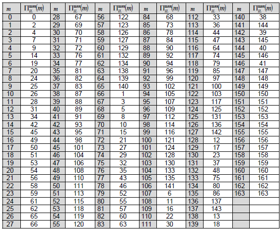
where ΠILmax(m) is given by Table 5.3.1.1-1 and KILmax = 164.
< 38.212-Table 5.3.1.1-1: Interleaving pattern ΠILmax(m) >
In Polar coding, some bit positions are more reliable than others. Interleaving ensures that the information bits are distributed in a way that maximizes the performance of the Successive Cancellation decoder.
How it Works:
- Bypass Mode: If the indicator IIL = 0, no interleaving occurs, and the output is identical to the input (Π(k) = k).
-
Interleaving Mode (IIL = 1):
- The system uses a master interleaving pattern ΠILmax(m) based on a maximum length of KILmax = 164.
- The algorithm iterates through this master pattern and selects indices that are valid for the current number of input bits (K).
- The formula Π(k) = ΠILmax(m) − (KILmax − K) maps the long master sequence down to your specific message length.
Interpretation of the code
Following is the interpretation of the codeblock
If IIL = 0:

  - No interleaving is applied.

  - Use identity mapping:

    Π(k) = k, for k = 0, 1, ..., K−1


Else (IIL = 1):

  - Build Π(k) by scanning the master pattern ΠILmax(m) (length KILmax = 164).

  - Initialize:

    k = 0

  - For each m = 0 to KILmax − 1:

    - Check if the master index is valid for current K:

      if ΠILmax(m) ≥ KILmax − K

        Π(k) = ΠILmax(m) − (KILmax − K)   // shift into [0 ... K−1]

        k = k + 1

      end if

    end for


Meaning:

  - Only the master indices in the range [KILmax − K ... KILmax − 1] are kept.

  - Subtracting (KILmax − K) renumbers that range into [0 ... K−1].
5.3.1.2 Polar encoding
The Polar sequence Q0Nmax−1 = {Q0Nmax, Q1Nmax, ..., QNmax−1Nmax} is given by Table 5.3.1.2-1, where 0 ≤ QiNmax ≤ Nmax − 1 denotes a bit index before Polar encoding for i = 0, 1, ..., Nmax − 1 and Nmax = 1024. The Polar sequence Q0Nmax−1 is in ascending order of reliability W(Q0Nmax) < W(Q1Nmax) < ... < W(QNmax−1Nmax), where W(QiNmax) denotes the reliability of bit index QiNmax.
For any code block encoded to N bits, a same Polar sequence Q0N−1 = {Q0N, Q1N, Q2N, ..., QN−1N} is used. The Polar sequence Q0N−1 is a subset of Polar sequence Q0Nmax−1 with all elements QiNmax of values less than N, ordered in ascending order of reliability W(Q0N) < W(Q1N) < W(Q2N) < ... < W(QN−1N).
Denote Q̄IN as a set of bit indices in Polar sequence Q0N−1, and Q̄FN as the set of other bit indices in Polar sequence Q0N−1, where Q̄IN and Q̄FN are given in Clause 5.4.1.1, |Q̄IN| = K + nPC, |Q̄FN| = N − |Q̄IN|, and nPC is the number of parity check bits.
Denote GN = (G2)⊗n as the n-th Kronecker power of matrix G2, where G2 = [ 1 0 1 1 ].
For a bit index j with j = 0, 1, ..., N − 1, denote gj as the j-th row of GN and w(gj) as the row weight of gj, where w(gj) is the number of ones in gj. Denote the set of bit indices for parity check bits as Q̄PCN, where |Q̄PCN| = nPC.
A number of (nPC − nPCwm) parity check bits are placed in the (nPC − nPCwm) least reliable bit indices in Q̄IN. A number of nPCwm other parity check bits are placed in the bit indices of minimum row weight in Q̄IN, where Q̄IN denotes the (|Q̄IN| − nPC) most reliable bit indices in Q̄IN. If there are more than nPCwm bit indices of the same minimum row weight in Q̄IN, the nPCwm other parity check bits are placed in the nPCwm bit indices of the highest reliability and the minimum row weight in Q̄IN.
Generate u = [u0 u1 u2 ... uN−1] according to the following:
k = 0;


if nPC > 0

  y0 = 0;  y1 = 0;  y2 = 0;  y3 = 0;  y4 = 0;


  for n = 0 to N − 1

    yt = y0;
y0 = y1;
y1 = y2;
y2 = y3;
y3 = y4;
y4 = yt;


    if n ∈ Q̄IN

      if n ∈ Q̄PCN

        un = y0;

      else

        un = c′k;

        k = k + 1;

        y0 = y0 ⊕ un;

      end if

    else

      un = 0;

    end if


  end for

else

  for n = 0 to N − 1

    if n ∈ Q̄IN

      un = c′k;

      k = k + 1;

    else

      un = 0;

    end if

  end for

end if
The output after encoding d = [d0 d1 d2 ... dN−1] is obtained by d = uGN. The encoding is performed in GF(2).
< 38.212-Table 5.3.1.2-1: Polar sequence Q0Nmax−1 and its corresponding reliability W(QiNmax) >


The provided images outline the final stages of the 5G NR Polar encoding process, specifically focusing on sub-channel classification, parity bit placement, and the final mathematical transformation into a codeword.
1. Sub-channel Reliability and Parity Placement
This stage determines which bit indices will carry data and where special parity check (PC) bits should be placed to improve decoding performance.
- Reliability Ranking: The system uses a master Polar sequence (Q0Nmax−1) of 1024 indices ranked by reliability. For a specific block size N, a subset (Q0N−1) is used, containing all indices less than N in ascending order of reliability.
-
Set Definition:
- Q̄IN: The set of bit indices chosen for information bits and parity check bits.
- Q̄FN: The remaining indices, which are frozen to zero.
Parity Check (PC) Placement: If nPC > 0, parity bits are distributed into two groups within the Q̄IN set:
- A portion (nPC − nPCwm) is placed in the least reliable indices of the set.
- The remaining bits (nPCwm) are placed in indices with the minimum row weight (w(gj)) in the generator matrix GN. If multiple indices have the same minimum weight, the ones with the highest reliability are chosen.
2. Codeword Generation Logic
This stage describes the algorithm to construct the input vector u and calculate the final output bits d.
-
Generating Vector u:
The algorithm iterates from n = 0 to N − 1 to fill each position un:
- Information Bits: If the index n is a data index (and not a parity index), un takes the next bit from the interleaved input sequence (c′k).
- Parity Bits: If n is a parity index (n ∈ Q̄PCN), un is calculated using a shifting parity logic (y-register update) to help the decoder.
- Frozen Bits: If the index n is not in Q̄IN, it is set to 0.
- The Final Transform: Once vector u is complete, the final encoded codeword d = uGN is obtained using the n-th Kronecker power of the kernel matrix: GN = (G2)⊗n. This matrix multiplication is performed in GF(2) (binary arithmetic).
Example 1 >
To visualize how the Generator Matrix (GN) is constructed, we use the Kronecker power (⊗) of the base kernel matrix G2.
1. The Base Kernel (G2)
The fundamental building block for all Polar codes in 5G NR is the 2 × 2 matrix:
G2 =
1
0
1
1
2. Building G4 (N = 4)
To get the matrix for N = 4, we take the Kronecker product of G2 with itself (G2 ⊗ G2):
G4 =
1
0
0
0
1
1
0
0
1
0
1
0
1
1
1
1
3. Building G8 (N = 8)
For N = 8, we repeat the process (G2 ⊗ G4). This creates a nested, fractal-like structure:
G8 =
1
0
0
0
0
0
0
0
1
1
0
0
0
0
0
0
1
0
1
0
0
0
0
0
1
1
1
1
0
0
0
0
1
0
0
0
1
0
0
0
1
1
0
0
1
1
0
0
1
0
1
0
1
0
1
0
1
1
1
1
1
1
1
1
Why this structure matters
- Row Weight (w(gj)): Notice that the rows have different numbers of ones (weights). For example, the first row has a weight of 1, while the last row has a weight of 8.
- Reliability Correlation: Generally, rows with higher weights correspond to more reliable “sub-channels”.
- Parity Placement: As seen in your provided images, 5G NR specifically places some parity check bits in the indices with the minimum row weight to optimize the code's distance properties.
The Final Codeword Calculation
Once you have your input vector u (which contains your data, parity bits, and zeros for frozen bits), the final output d is simply:
d = u · GN (mod 2)
Each bit di in the final codeword is an XOR combination of specific input bits in u.
Example 2>
Let's apply the NR Polar Encoding logic to a concrete example. We will encode a small 2-bit message (K = 2) into a 4-bit mother code (N = 4).
1. The Inputs
- Information Bits (c): [c0, c1] = [1, 0].
- Interleaving: Assuming IIL = 0, the interleaved sequence c′ = [1, 0].
- Parity Bits: We will assume nPC = 0 for this simple example.
- Reliability Indices: For N = 4, let's assume the reliability ranking is Q = {0, 1, 2, 3} (from least to most reliable).
2. Constructing Vector u
We need to fill the 4 positions of u = [u0, u1, u2, u3]. Since K = 2, we pick the 2 most reliable indices for data and freeze the rest.
- Most Reliable Indices: {2, 3} (Data Set Q̄I4).
-
Frozen Indices: {0, 1} (Frozen Set Q̄F4).
| Index (n) | Type | Value Calculation | Result |
|---|---|---|---|
| u0 | Frozen | Set to 0 | 0 |
| u1 | Frozen | Set to 0 | 0 |
| u2 | Data | First info bit c′0 | 1 |
| u3 | Data | Second info bit c′1 | 0 |
Vector u = [0, 0, 1, 0]
3. The Transformation (d = u · G4)
Now we multiply our vector u by the G4 matrix we constructed earlier using binary (XOR) arithmetic:
d = [0, 0, 1, 0] ·
1
0
0
0
1
1
0
0
1
0
1
0
1
1
1
1
Calculating each bit of d:
d0 = (0·1) ⊕ (0·1) ⊕ (1·1) ⊕ (0·1) = 0 ⊕ 0 ⊕ 1 ⊕ 0 = 1d1 = (0·0) ⊕ (0·1) ⊕ (1·0) ⊕ (0·1) = 0 ⊕ 0 ⊕ 0 ⊕ 0 = 0d2 = (0·0) ⊕ (0·0) ⊕ (1·1) ⊕ (0·1) = 0 ⊕ 0 ⊕ 1 ⊕ 0 = 1d3 = (0·0) ⊕ (0·0) ⊕ (1·0) ⊕ (0·1) = 0 ⊕ 0 ⊕ 0 ⊕ 0 = 0
Final Codeword d = [1, 0, 1, 0]
Summary of the result
The message "10" was transformed into the codeword "1010".
- Even though we only sent 2 bits of info, every bit in the output d is now mathematically tied to the input bits based on the structure of the generator matrix.
- The receiver uses this structure and the known "0" values at positions u0 and u1 to work backward and correct errors.
Reference
[1] 3GPP TSG RAN WG1 #86 - R1-166414 Discussion on LDPC codes for NR
[2] 3GPP TSG RAN WG1 #86 R1-166769 Discussion on Length-Compatible Quasi-Cyclic LDPC Codes
[3] 3GPP TSG RAN WG1 #86 R1-166770 Discussion on Rate-Compatible Quasi-Cyclic LDPC Codes
[4] 3GPP TSG RAN WG1 #86 R1-166929 LDPC Code Design for NR
[6] 3GPP TSG RAN WG1 #86 R1-167889 Design of Flexible LDPC Codes