Precoding is the one block in the downlink chain that resists a plain language description. Every other block moves data from one form to another. This one mixes the layers together, and the mixing rule is a matrix that can change from one transmission to the next.

Unfortunately I don't know how to explain this part in plain language without using any mathematical tools.

As you see in the following diagram, Precoding is the process that is between Layer Mapper and Resource mapper. In practice, this precoding is the process in which the incoming data (=output of layer mapper) are distributed to each antenna ports. Then the question is "How each of the data (layered data) get distributed to each of antenna ports ?". Is it as simple like "data on layer 0 goes blindly to antenna port 1 and data on layer 1 goes blindly to antenna port 1". Unfortunately it is not that simple. In reality, the data from all the layers gets combined in specify way and then those combined data gets distributed to each of the antenna port. so we can roughly say "Each antenna ports carries at least some portions of data from all the layers".

Then the question is "How (in what kind of rule) the data from all the layers get combined ?". The rule is defined by a precoding matrix that we will look into, in this page.

Followings are the topics to be covered in this page.

• Overall Process
• Precoding vs Transmission Mode
• Precoding for Transmit Diversity
• Precoding for Spatial Multiplexing - Precoding with large delay CDD
• Precoding for Spatial Multiplexing - Precoding with the selected Codebook
•   Codebook selection for Precoding - 2 Antenna Ports
•   Codebook selection for Precoding - 4 Antenna Ports
•   Codebook for 4 x 2 MIMO
•   Precoding Information Field
•   36.212 Table 5.3.3.1.5-4: Content of precoding information field for 2 antenna ports
•   36.212 Table 5.3.3.1.5-5: Content of precoding information field for 4 antenna ports
• Tutorials on complex transformation
• Reference

Overall Process

First I would suggest you to get a big picture on the role of the Procoding on the overal downlink physical layer process as highlighted below.  One thing very tricky about Precoding in LTE is that there are so many variations and is very hard to figure out which one to be applied to which case. Just taking a look at the list of sub titles listed below whenever you have chance. If you go through this list more than 10 or 20 times, you would have some image on several different cases where different variations of precoding is used.

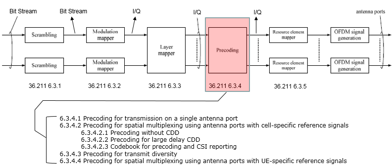
The chain with 6.3.4 opened up. One block in the drawing, and five separate rules inside it.

• The highlighted box is the only one with a red clause number. Every other block carries a black one: 6.3.1 for Scrambling, 6.3.2 for the Modulation mapper, 6.3.3 for the Layer mapper and 6.3.5 for the Resource element mapper.
• The labels above the chain change at the Modulation mapper. Bit Stream on the left, I/Q from there onward, and antenna ports at the right edge.
• The list underneath has five entries, and only one of them applies to any given transmission. 6.3.4.1 is the single antenna port case, 6.3.4.3 is transmit diversity, and 6.3.4.2 with its three sub-entries is spatial multiplexing.
• 6.3.4.4 sits at the foot of the list and this page does not cover it. It is spatial multiplexing again, built on UE-specific reference signals rather than cell-specific ones.

That list is the reason the page runs long. Four of the five entries are separate precoding rules, and the precoder does not choose between them on its own. The transmission mode decides, and the next section is the table that maps one to the other.

One distinction inside the list is easy to miss. 6.3.4.2 and 6.3.4.4 are both spatial multiplexing, and they differ only in which reference signal the receiver estimates the channel from. Cell-specific reference signals go with 6.3.4.2 and with most of the transmission modes below. UE-specific reference signals go with 6.3.4.4.

• Precoding is one block and five rules : the drawing shows a single box, and the list under it shows how many different things that box can be.
• The clause number names the case : 6.3.4.1 for one antenna port, 6.3.4.3 for transmit diversity, and 6.3.4.2.x for spatial multiplexing.
• The transmission mode picks the rule : nothing in the chain around the precoder changes, so the mode is where the choice is actually recorded.

Precoding vs Transmission Mode

Each of those variants of the precoding can be mapped to each of Transmission Mode and the number of Antenna also influence on which type of procoding will be used in a specific situation of Transmission Mode.  Also, go through the following table whenever you have chance.

Every transmission mode against the precoding clause it uses. The Precoding column is the one to read first, because it names the sub-clause each of the sections below covers.

Reading the Precoding column downward shows how few rules there really are. 6.3.4.3 appears in TM2, TM3, TM5, TM7 and TM8, and in every one of those it is the single codeword row. Transmit diversity is what a two antenna mode falls back to when it has only one transport block to send.

The Codebook column splits the same way. It reads N/A wherever transmit diversity is in force, because that rule builds its own matrix and never consults a codebook. It names Table 6.3.4.2.3-1 wherever spatial multiplexing is in force, and TM3 is the row where the entry is fixed rather than chosen.

• N/A in the Codebook column is a real answer : transmit diversity and the single antenna port case both construct their matrix from the clause alone.
• TM3 fixes the codebook entry : large delay CDD uses {number of layers, codebook index} = {2, 0} and nothing else, so no feedback is needed to pick it.
• TM4 is where the UE gets a say : four entries are available at one layer and two at two layers, and the reported PMI chooses among them.
• TM1 is the only single antenna row : every other mode in the table lists 2 in the antenna column, which is why the codebook sections below start from two ports.

Precoding for Transmit Diversity

Following is the case where a single layer data stream gets transmitted by two antenna. Overall procedure is as follows. (TM2, TM6 is using this configuration)

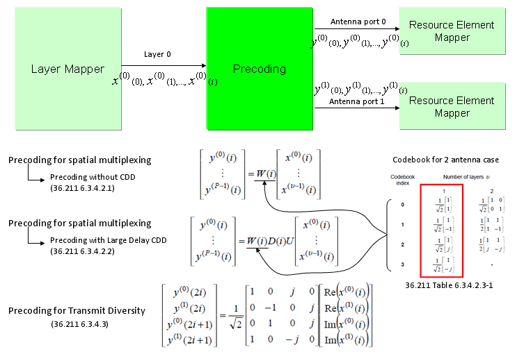
One layer in, two antenna ports out, with all three precoding equations set side by side underneath.

• The top of the drawing carries a single arrow labelled Layer 0 into the Precoding box, and two arrows out of it labelled Antenna port 0 and Antenna port 1.
• The three equations underneath are the three rules. Spatial multiplexing without CDD is y = W(i)x, large delay CDD is y = W(i)D(i)Ux, and transmit diversity is the fourth equation with the explicit 4 by 4 matrix.
• Only the transmit diversity equation names its matrix in full. It reads 1/√2 times a matrix of 1, 0, j and -1 entries, and it takes Re(x) and Im(x) as separate inputs.
• That equation produces y(2i) and y(2i+1) for both antenna ports at once. Two output symbols per port come from one pair of input symbols, which no other rule on this page does.
• The codebook at the right is 36.211 Table 6.3.4.2.3-1, and the red box marks the layer 1 column. Transmit diversity does not use it, and the sections below do.

If we apply the Layer 1 code book to a sequence of data, we will get the constellation as follows. If you briefly see the constellation, you don't find any differences in terms of constellation except overall amplitude gets smaller after going through the precoding block. But if you following through the precoding process for each one (single) constellation, you will understand the differences.

The Octave code is here. (I create this code in Octave which is a Matlab like GNU program,but I guess it will run in Matlab without any modification. I tried to write the code so that I can run on both program but I haven't tested it in Matlab myself).  

In addition, I posted another type of tutorials that may help you with intuitive understandings on this kind of complex number operation. See my visual note [Matrix Complex] (this, this, this, this) to build up intuition.

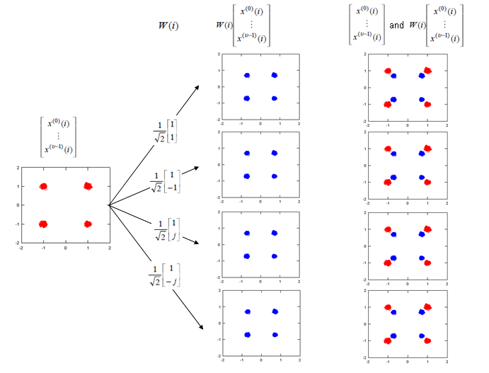
All four one layer entries applied to the same input. The four outputs are the same four points, turned by a different angle each time.

NOTE : If I expand the transformation shown above into two antenna case (diversity) to give you more concrete idea, it can be illustration as follows. Since all of the data used here are complex numbers (Real = I, Imaginary = Q), the result of operation may not be so intuitive to you. If you are really interested in understanding the result of transformation, try this transformation with your own program or pen-paper calculation on your own. At least, play with the matlab code that I created and linked here.

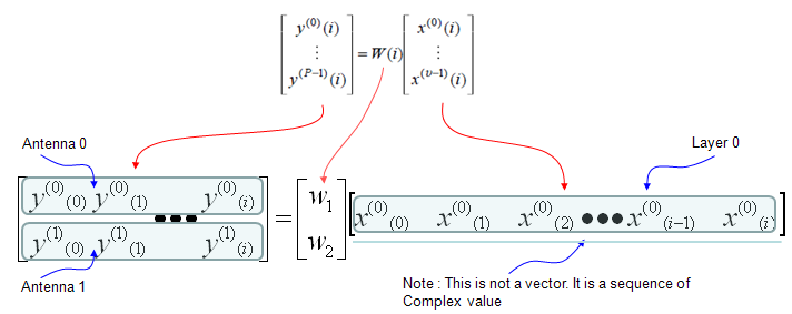
The same equation with the sequences drawn out. The note at the lower right is the point: x is a sequence of complex values rather than a vector.

• The left side stacks two rows labelled Antenna 0 and Antenna 1, each running y(0), y(1) up to y(i).
• The right side has one row labelled Layer 0, running x(0), x(1), x(2) up to x(i).
• The matrix between them is a column of two entries, W1 and W2. One layer in and two antennas out is what makes it a column rather than a square.
• The note at the lower right warns against reading the x row as a vector. Each element is one complex value, and the precoding matrix is applied to them one at a time.

Precoding for Spatial Multiplexing - Precoding with large delay CDD

Large delay CDD is the spatial multiplexing rule that asks the UE for nothing. The matrix is fixed by the specification, and two further matrices in front of it keep the mapping moving, so no layer sits on a bad path for long. The drawing below is the transmitter and the receiver together, and there is no feedback arrow anywhere in it.

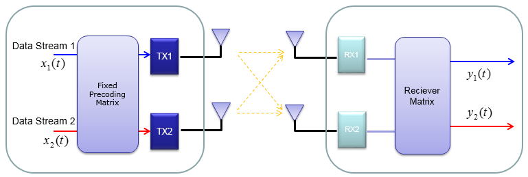
The open loop arrangement. The precoding matrix is marked Fixed, and nothing runs backward from the receiver to the transmitter.

• Data Stream 1 and Data Stream 2 enter on the left as x₁(t) and x₂(t), and both go into the one block labelled Fixed Precoding Matrix.
• TX1 and TX2 leave that block, and the dashed paths between the antennas cross. Each receive antenna hears both transmit antennas, which is the reason a matrix is needed at all.
• The Reciever Matrix on the right undoes the mixing and produces y₁(t) and y₂(t). The spelling is the drawing’s own.
• The word Fixed is the whole difference from the next section. Compare this drawing with the one that opens the codebook section, which adds a return path.

To make the process and understanding simpler, let's assume that we are only focusing on two antenna case. If it is two antenna case, the block diagram around the Precoding looks as follows. (TM3 is using this configuration)

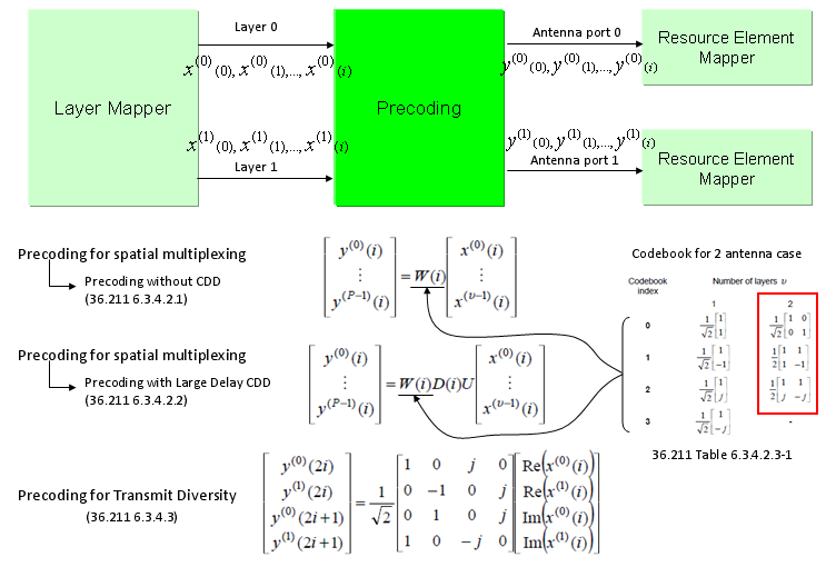
The same three equations as before, now with two layers arriving instead of one. The red box has moved to the two layer column.

• Layer 0 and Layer 1 both enter the Precoding box, and Antenna port 0 and Antenna port 1 both leave it. Two in and two out is what makes the precoding matrix square here.
• The red box in the codebook now marks the layers = 2 column rather than the layers = 1 column, so the entries in play are the 2 by 2 ones.
• The middle equation is the one this section is about. It reads y = W(i)D(i)Ux, and the two extra matrices sit between W(i) and the layer data.

In case of Procoding with Large Delay CDD, two additional matrix are multiplied before it is multiplied by Procoding matrix as shown below. Please keep in mind the role of each matrix in the equation. (Refer to CDD page if you want to know further details of CDD concept itself)

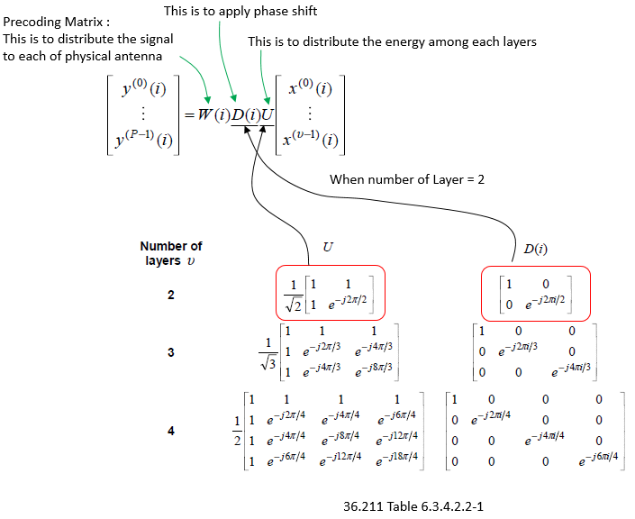
36.211 Table 6.3.4.2.2-1 under the equation it belongs to. Three matrices multiply in a row, and the annotations say what each one is for.

• The leftmost note reads Precoding Matrix, this is to distribute the signal to each of physical antenna, and its arrow lands on W(i).
• The middle note reads this is to apply phase shift and points at D(i). D(i) is diagonal, and its entries are powers of e^-j2π/υ.
• The right note reads this is to distribute the energy among each layers and points at U. U is full rather than diagonal, so every layer reaches every output of that stage.
• The table gives U and D(i) for 2, 3 and 4 layers. The red boxes mark the 2 layer row, which is the case the annotation When number of Layer = 2 points at.
• Only D(i) carries the index i. W and U do not, so the time variation in this rule comes from one matrix alone.

Then a question would come up. Where is W(i) matrix defined ? One or a couple of specially selected matrix from the codebook are used. Which matrix (which index) of the codebook is used are defined in the 36.211 as shown below.

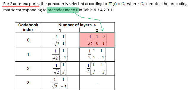
36.211 6.3.4.2.2, the two antenna port sentence. One codebook entry is named, and there is nothing to choose.

• The highlighted words are precoder index 0, and the red box marks that entry in the layers = 2 column of Table 6.3.4.2.3-1.
• The boxed matrix is 1/√2 times the identity. For two antenna ports the precoding matrix of this rule does no mixing of its own, and D(i) and U do all the work.
• The table underneath is the same Table 6.3.4.2.3-1 that the codebook sections below return to. Here only one of its eight entries is reachable.

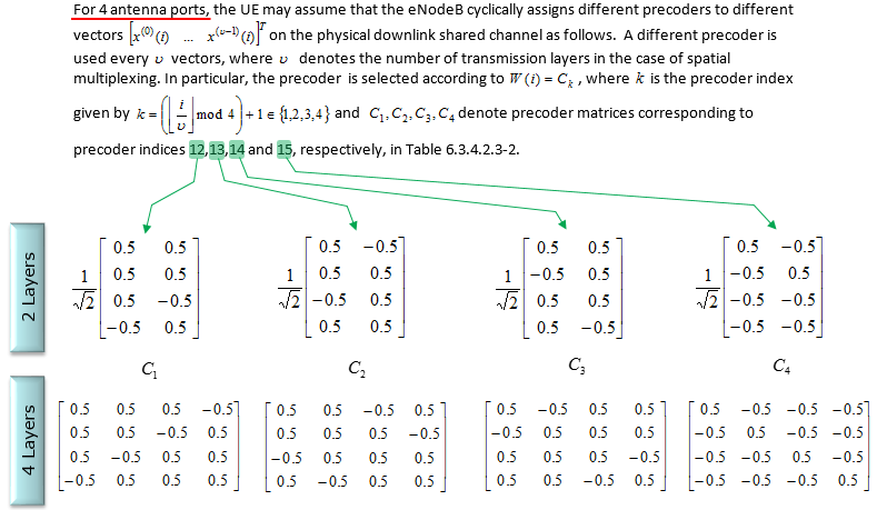
36.211 6.3.4.2.2 again, this time for four antenna ports. Four matrices are named instead of one, and the transmitter cycles through them.

• The highlighted indices are 12, 13, 14 and 15 in Table 6.3.4.2.3-2, and they are named C₁ to C₄ in the drawing.
• The index is k = (floor(i/υ) mod 4) + 1, so the precoder changes every υ vectors and repeats every four changes.
• The upper row draws the four matrices at 2 layers, each 4 by 2 and scaled by 1/√2. The lower row draws them at 4 layers, each 4 by 4 with no scaling shown.
• Every entry in all eight matrices is plus or minus 0.5. The four matrices differ only in the pattern of signs, which is what makes cycling through them cheap.

The only way to understand this concept to the skin would be to try this yourself and play with all these parameters like your toys. To help this, I created a small octave code and attached here. (I create this code in Octave which is a Matlab like GNU program, but I guess it will run in Matlab without any modification. I tried to write the code so that I can run on both program but I haven't tested it in Matlab myself).

I posted another type of tutorials that may help you with intuitive understandings on this kind of complex number operation. See my visual note [Matrix Complex] (this, this, this, this) to build up intuition.

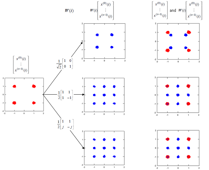
What a precoding matrix does to a constellation. The input is the red four point plot on the left, and each row applies a different matrix to it.

• The left plot is the input, four red points at the QPSK positions near plus and minus 1 on both axes.
• The top row applies 1/√2 times the identity. The output is still four points, moved inward to about plus and minus 0.7.
• The two lower rows apply the 2 by 2 entries of the codebook. Both produce nine points rather than four, because two layers are being summed into one antenna port.
• The right column overlays input and output on the same axes. The point to take is that the amplitude shrinks in every case, and the shape changes only when the matrix mixes two layers.

Note : If I expand the transformation shown above into a 2 x 2 case to give you more concrete idea, it can be illustration as follows. Since all of the data used here are complex numbers (Real = I, Imaginary = Q), the result of operation may not be so intuitive to you. If you are really interested in understanding the result of transformation, try this transformation with your own program or pen-paper calculation on your own. At least, play with the matlab code that I created and linked here.

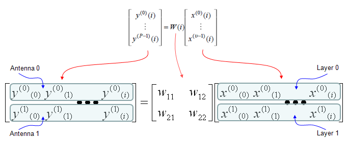
The two layer version of the same expansion. The matrix is square here, and that is the only structural change.

• The right side now carries two rows, Layer 0 and Layer 1, where the one layer version carried a single row.
• The matrix in the middle has four entries, W₁₁ to W₂₂, rather than the column of two.
• The left side is unchanged at two rows, Antenna 0 and Antenna 1. The antenna count did not move, so only the input side grew.

Following is the real Downlink signal coming out of a LTE network emulator. I capture the signal and analyzed it with a vector spectrum analyzer with LTE analysis functionality.

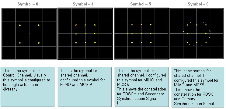
A live downlink, symbol by symbol. The constellation changes across the subframe because different symbols carry different channels.

• Symbol 0 shows four points. The note underneath says it is the control channel, usually configured for single antenna or diversity.
• Symbols 4, 5 and 6 show more than four points. All three notes say MIMO and MCS 9, which is the shared channel.
• Symbol 5 also carries the Secondary Synchronization Signal and symbol 6 the Primary Synchronization Signal, which is why those two look less regular than symbol 4.
• The picture is a capture rather than a calculation, so the clouds are spread by noise. The count of clusters is what to read, not their tightness.

Now let try apply the CDD. I would recommend you to try investigate on what's is CDD in practical sense and what would be the advantage of applying CDD. Here I would only show you the result of the CDD application. The Octave code is here. (I create this code in Octave which is a Matlab like GNU program, but I guess it will run in Matlab without any modification. I tried to write the code so that I can run on both program but I haven't tested it in Matlab myself). I posted another type of tutorials that may help you with intuitive understandings on this kind of complex number operation. See my visual note [Matrix Complex] (this, this, this, this) to build up intuition.

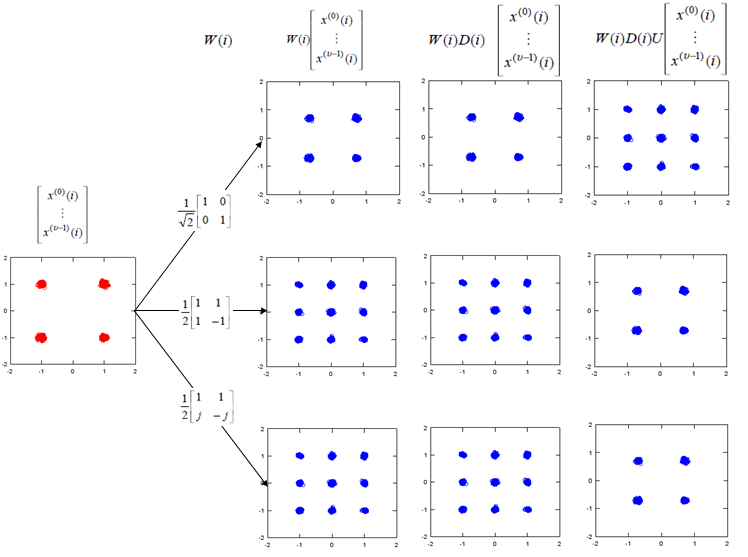
The same experiment with the CDD matrices added one at a time. Each column to the right multiplies in one more matrix.

• The first column is W(i) alone and repeats the plots above. The second adds D(i) and the third adds U.
• In the top row the point count goes 4, then 4, then 9. D(i) only rotates, so it cannot change how many distinct points there are, and U is what mixes the layers.
• In the two lower rows the count goes 9, then 9, then 4. There the matrix already mixed the layers, and U undoes enough of it to collapse the constellation back.
• Reading across rather than down is the useful direction here. Each step to the right is one more matrix in the product, in the order the equation writes them.

Precoding for Spatial Multiplexing - Precoding with the selected Codebook

The rule in this section keeps the same equation as the one before it, y = W(i)x, and changes where W(i) comes from. The UE measures the channel, picks the entry it would prefer, and reports the index. Both ends already hold the table, so the report is a few bits rather than a matrix.

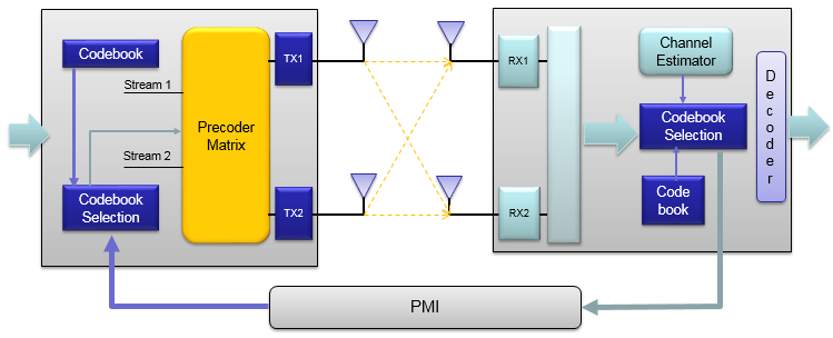
The closed loop arrangement. The bar along the foot marked PMI is what the previous section did not have.

• Both ends hold a block marked Codebook. The receiver selects from its copy and the transmitter looks the choice up in its own.
• The Channel Estimator at the receiver feeds Codebook Selection. The choice is made where the channel is measured, not where the data is sent.
• The PMI bar runs along the bottom from the receiver back to Codebook Selection at the transmitter. That return path is the whole difference from the open loop drawing above.
• The Precoder Matrix block is drawn in yellow and takes Stream 1 and Stream 2. What changes between transmissions is the matrix it holds, not the wiring around it.

• Closed loop means one number travels back : the UE reports an index into a shared table, and no matrix is ever sent over the air.
• The equation does not change : y = W(i)x here as well, with neither D(i) nor U in the product.
• The eNB is not bound by the report : the PMI is a preference, and the precoding information field in the grant is what actually states the matrix used.

< Codebook selection for Precoding - 2 Antenna Ports >

Getting one step deeper into the procedure, you may have a question asking "Which code book matrix (W(i)) do we have to use for each DL transmission ?". I think following table (Table 6.3.4.2.3-1 from 36.211) and the comments would answer the question.

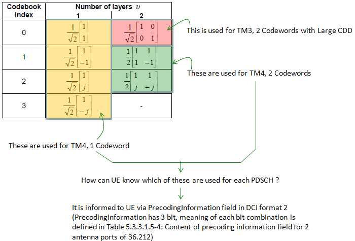
36.211 Table 6.3.4.2.3-1 with each group coloured by the mode that uses it. Eight entries in total, and no mode reaches all of them.

• The yellow column is layers = 1 and holds four entries, indices 0 to 3. The note says these are used for TM4, 1 Codeword.
• The green pair is layers = 2 at indices 1 and 2. The note says these are used for TM4, 2 Codewords.
• The red cell is layers = 2 at index 0, and the note says it is used for TM3, 2 Codewords with Large CDD. It is the entry the previous section named.
• The layers = 2 cell at index 3 is a dash. Only three of the four indices have a two layer entry, so the table holds eight matrices rather than the eight the grid suggests.
• The question at the foot asks how the UE knows which is used, and the answer written under it names the PrecodingInformation field in DCI format 2 and 36.212 Table 5.3.3.1.5-4.

Even though we can use any of the items in this table, NW can specify which of the items will be used for each user(each connection) by defining codebookSubsetRestriction IE in .radioResourceConfigDedicated.physicalConfigDedicated.antennaInfo.

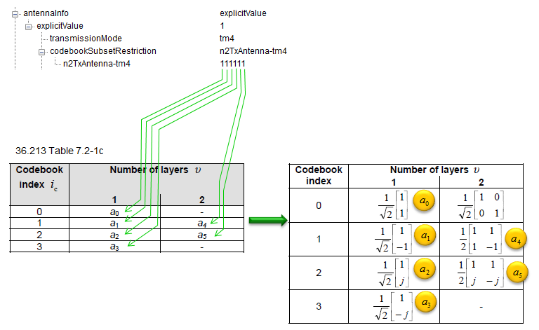
A capture of codebookSubsetRestriction, with each bit traced to the codebook entry it enables. The value shown is one network’s setting, not a specification default.

• The tree reads antennaInfo, explicitValue, transmissionMode tm4, then codebookSubsetRestriction with n2TxAntenna-tm4 set to 111111.
• Six bits map to six entries because 36.213 Table 7.2-1c labels them a₀ to a₅. Four sit in the layers = 1 column and two in the layers = 2 column.
• All six bits are 1 in this capture, so nothing is restricted. Every entry the mode allows is available to the UE.
• The dashes in the table are why there are six labels and not eight. Indices 0 and 3 have no two layer entry to restrict.

< Codebook selection for Precoding - 4 Antenna Ports >

Four antenna ports need a much larger table, and it is not written the same way. The two port table lists the matrices themselves. This one lists a generating vector for each index and leaves the matrix to be computed, which is what the worked example below does.

Following is from Table 6.3.4.2.3-2 of 36.211 (Table 6.3.4.2.3-2 Codebook for transmission on antenna ports {0,1,2,3}).

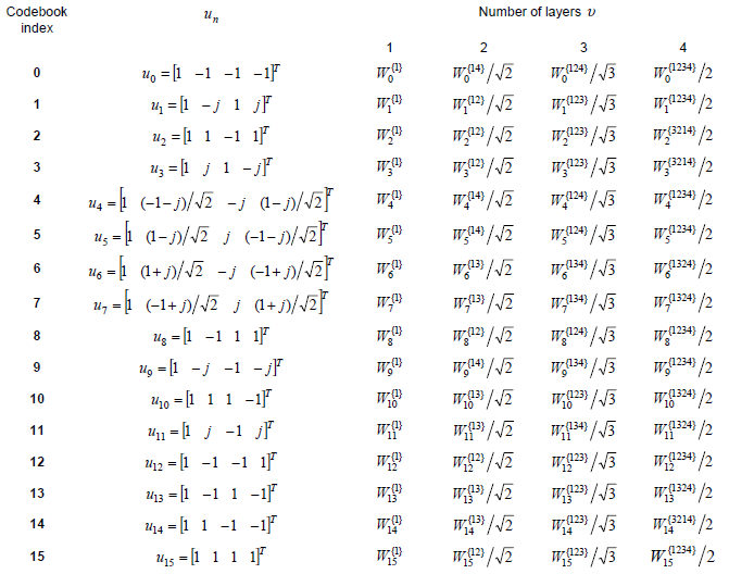
36.211 Table 6.3.4.2.3-2. Sixteen indices, and not one matrix printed anywhere in it.

• The second column gives u_n for each index. Indices 0 to 3 and 8 to 15 use entries of 1, -1, j and -j only, while 4 to 7 bring in (1±j)/√2 terms.
• The four right columns are headed 1, 2, 3 and 4 under Number of layers. Every cell there is a W with a superscript and a divisor.
• The superscript is a list of column numbers. W₀⁽¹⁴⁾ means take columns 1 and 4 of W₀, and the divisor √2 matches the two columns taken.
• The divisors run 1, √2, √3 and 2 across the four columns, which is the square root of the layer count each time.

How to interpret this table ? I took me pretty long time to figure it out. You would not get the Precoding Matrix directly from this table. You need to go through a couple of intermediate steps before you get the matrix.

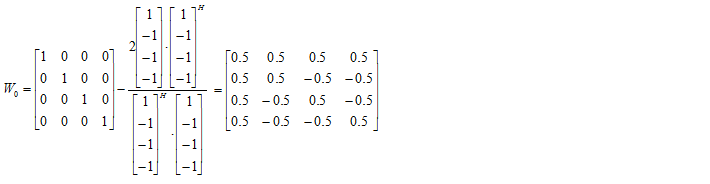
First, you have to use following equation to calculate Wn. (Here you see a special symbol called 'Hermitian'. If you are not familiar with this, refere to Hermitian Matrix page)

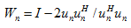
Let's take u0 case as an example. u0 is defined as follows according to Table 6.3.4.2.3-2 of 36.211.

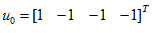
By plugging this into the Wn expression, you would get the result as follows.

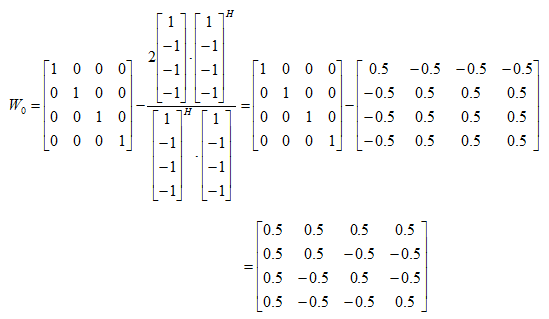
Once you get the Wn, getting W matrix for one, two, three, four antenna case is almost automatic. I think just following illustration would be self-explanatory (I hope -:)).

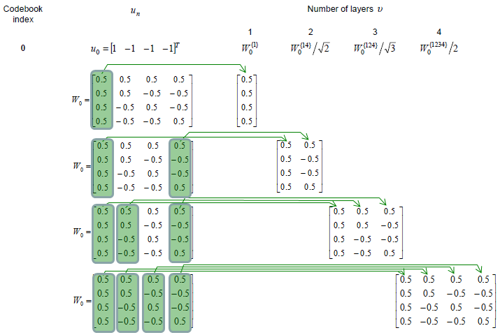
How a superscript becomes a matrix. Each row takes a different set of columns out of the same W₀.

• The top row takes column 1 alone and produces the layers = 1 entry, a single column of four 0.5 values.
• The second row shades columns 1 and 4 and produces the layers = 2 entry, which is the (14) in the superscript read literally.
• The third row shades columns 1, 2 and 4 for (124), and the fourth shades all four for (1234).
• W₀ itself is redrawn on each row and never changes. Only the shading moves, which is the point the figure is making.

The equation above it is a Householder transformation. Each W_n is built by subtracting a scaled outer product from the identity. One property of that construction shows up in every matrix on this page. The diagonal is 0.5 throughout, because u^Hu is 4 for every generating vector in the table.

Two things follow from the table being written this way. The codebook holds sixteen vectors rather than sixty four matrices, and the same W_n serves all four layer counts. Neither is visible if the table is read as a list of matrices.

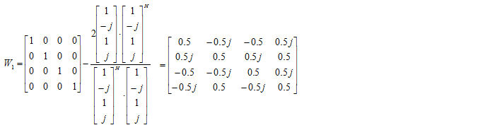
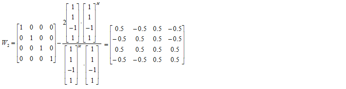
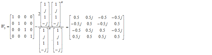
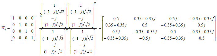
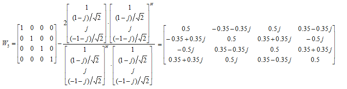
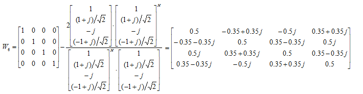
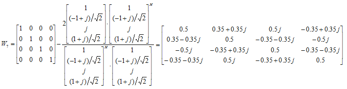
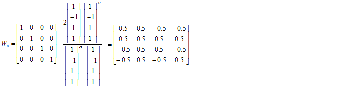
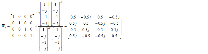
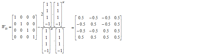
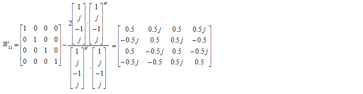
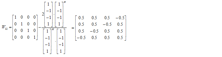
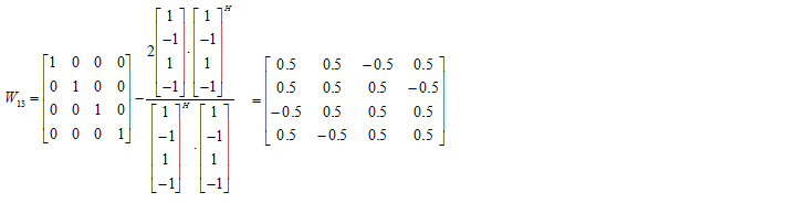
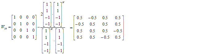
Following is Wn that I calculated for all the codebook index. (You can get the Octave code that I used here. I haven't tried with Matlab.. it is up to you checking it with Matlab). I will leave it up to you to figure out all the W matrix for one, two, three, four antenna on your own. You would never know what you don't know until you try on your own.

Codebook Ind	Wn
0
1
2
3
4
5
6
7
8
9
10
11
12
13
14
15

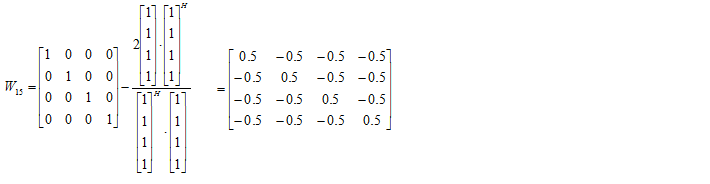W_n worked out for all sixteen codebook indices of 36.211 Table 6.3.4.2.3-2. Each row shows the Householder construction on the left and the resulting 4 by 4 matrix on the right.

• The identity and the generating vector are redrawn on every row, so the only thing that changes down the table is u_n.
• Eight of the sixteen come out purely real, with every entry at plus or minus 0.5: indices 0, 2, 8, 10, 12, 13, 14 and 15. The other eight come out complex, because their generating vectors carry a j or a (1±j)/√2 term.
• The diagonal reads 0.5 in all sixteen matrices. That is the Householder construction showing through, and it is a quick way to check a hand calculation.

< Codebook for 4 x 2 MIMO >

The table above lists W_n at full size. Four antennas sending two layers needs the two column version instead, so the column pair named in the superscript is pulled out and rescaled. The table below does that for all sixteen indices.

Codebook Index	Wn
0
1
2
3
4
5
6
7
8
9
10
11
12
13
14
15

The same sixteen indices reduced to two columns. The shaded columns on the left are the ones the superscript names, and the 1/√2 on the right is the rescaling that goes with taking two of four.

• Each row states the superscript it is expanding. Index 0 is W₀⁽¹⁴⁾, so columns 1 and 4 are shaded, and index 15 is W₁₅⁽¹²⁾, so columns 1 and 2 are.
• The shaded pairs are not the same from row to row. Reading the superscripts down the table is the only way to know which pair applies, and Table 6.3.4.2.3-2 is where they come from.
• Every result is 4 rows by 2 columns. Four rows because there are four antenna ports, and two columns because there are two layers.

Precoding Information Field

In previous sections, you have seen so many different precoding matrix. Then you may have ask "How eNB can inform of which matrix it used ?" or "How a UE can figure out which precoding matrix is used ?".

eNodeB can inform UE of which codebook index is used by setting the PrecodingInformation field in DCI format 2 or 2A.

< 36.212 Table 5.3.3.1.5-4: Content of precoding information field for 2 antenna ports >

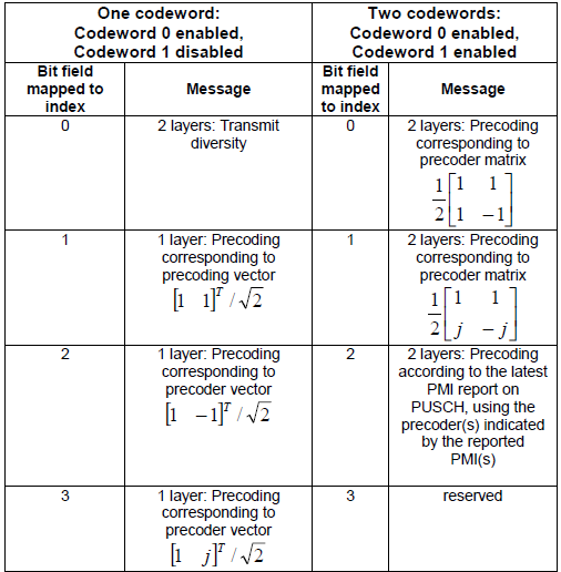
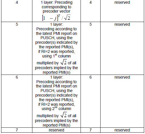
36.212 Table 5.3.3.1.5-4 across both screenshots. Three bits, eight values, and two completely different meanings depending on how many codewords are enabled.

• The table splits into One codeword and Two codewords, and the same bit value means different things on the two sides.
• Value 0 with one codeword reads 2 layers: Transmit diversity. That is how a two antenna mode signals the fallback the transmission mode table showed.
• Values 1 to 4 with one codeword each name a precoder vector in full: [1 1]^T, [1 -1]^T, [1 j]^T and [1 -j]^T, all divided by √2. They are the layers = 1 column of Table 6.3.4.2.3-1.
• Values 0 and 1 with two codewords print the 2 by 2 matrices ½[1 1; 1 -1] and ½[1 1; j -j]. Those are the two green entries in the coloured table earlier on this page.
• Values 2, 5 and 6 do not name a matrix at all. The cell text reads “Precoding according to the latest PMI report on PUSCH”, so the grant points back at the UE’s own report rather than carrying the answer.
• Value 7 is reserved on both sides, and with two codewords so are 3 to 7. Three bits are more than that half of the table needs.

< 36.212 Table 5.3.3.1.5-5: Content of precoding information field for 4 antenna ports >

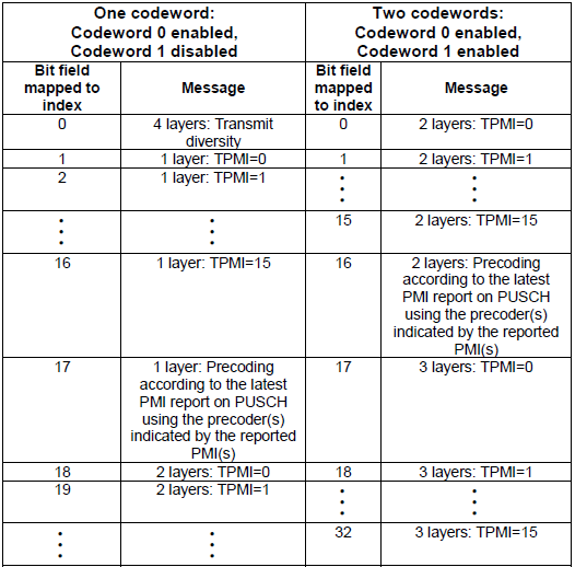
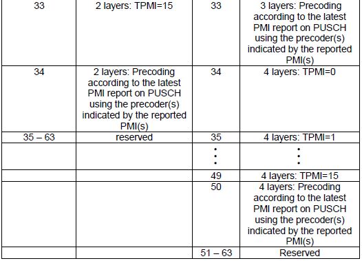
36.212 Table 5.3.3.1.5-5 across both screenshots. Four antenna ports need six bits, and the field stops naming matrices and starts naming TPMI values.

• The one codeword side runs 0 for 4 layers transmit diversity, then 1 to 16 for 1 layer with TPMI 0 to 15, then 18 to 33 for 2 layers with TPMI 0 to 15.
• The two codeword side runs 0 to 15 for 2 layers, 17 to 32 for 3 layers and 34 to 49 for 4 layers, each with TPMI 0 to 15.
• TPMI is the codebook index in Table 6.3.4.2.3-2, which is the sixteen entry table this page worked through. Sixteen values is exactly four bits of the six.
• One value in each block points at the PMI report instead of a TPMI: 17 and 34 on the one codeword side, and 16, 33 and 50 on the two codeword side.
• The rest is reserved, 35 to 63 on the one codeword side and 51 to 63 on the other.

The arithmetic behind the field width is worth doing once. Two antenna ports need three bits because eight values cover the four single layer entries, the two layer entries and the PMI cases. Four antenna ports need six, because sixteen TPMI values have to be spelled out for each supported layer count.

36.212 adds one restriction that the screenshots do not show. Indices 18 to 34 on the single codeword side are only supported for a retransmission, and only when that transport block was first sent on two layers with closed loop spatial multiplexing. A two layer entry with one codeword enabled is a retransmission signal rather than a new grant.

Reading the two tables together settles the question the section opened with. The UE never has to guess which matrix was used. Either the field names it outright, or it names the report the UE itself sent, and both cases are unambiguous at the receiver.

• The same bits mean different things : the codeword count comes from elsewhere in the DCI, and the precoding information field cannot be read without it.
• Two ports name matrices, four ports name indices : 36.212 prints the actual vectors for two antenna ports and falls back to TPMI once there are sixteen of them.
• Some values point back at the UE : one code point in each block defers to the latest PMI report instead of naming a matrix, and that is how closed loop normally runs.
• Transmit diversity has its own code point : value 0 with one codeword, in both tables, which is how the fallback in the transmission mode table is actually signalled.

Tutorials on complex transformation

As I mentioned above, if you just see the overall constellation, you don't find any differences in terms of constellation except overall amplitude gets smaller after going through the precoding block. But if you following through the precoding process for each one (single) constellation, you will understand the differences. Following sequences of plots shows you 'Precoding' result of each points with each precoding (transformation) vector. Colored spots represents the constellation (I/Q data) coming(I/Q data) out of Layer Mapping block and coming into Precoding block. Black spots represents the constellation coming out of the Precoding block. You would notice that each of the colored spots creates two black spots. Even for the plot with only one black spots, it is the superimposed result of two black spots. Each of the black spots gets transmitted by each of the antenna.

The Octave code is here. (I create this code in Octave which is a Matlab like GNU program, but I guess it will run in Matlab without any modification. I tried to write the code so that I can run on both program but I haven't tested it in Matlab myself).

I posted another type of tutorials that may help you with intuitive understandings on this kind of complex number operation. See my visual note [Matrix Complex] (this, this, this, this) to build up intuition

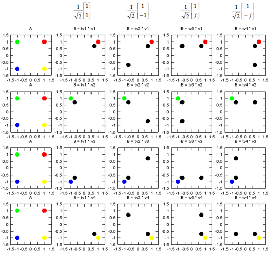
One complex multiplication at a time. Each row fixes an input point and each column fixes a vector, so the black dot is the result.

Followings are short description for each of dots (v) and vectors(tv).

• Red Dot = v1 (a complex number)
• Green Dot = v2 (a complex number)
• Blue Dot = v3 (a complex number)
• Yellow Dot =v4 (a complex number)
• Black Dot = the result of math operation (e.g, tv1 * v1,tv2 * v1,tv3 * v1,tv4 * v1)
• 1/2[1;1] = tv1 (a 2x1 complex vector)
• 1/2[1;-1] = tv2 (a 2x1 complex vector)
• 1/2[1;j] = tv3 (a 2x1 complex vector)
• 1/2[1;-j] = tv4 (a 2x1 complex vector)

Reference

• TS 36.211 v19.3.0 (Release 19) - E-UTRA Physical channels and modulation. Clause 6.3.4 Precoding, and the codebook tables 6.3.4.2.2-1, 6.3.4.2.3-1 and 6.3.4.2.3-2.
• TS 36.212 v19.3.0 (Release 19) - E-UTRA Multiplexing and channel coding. Clause 5.3.3.1.5 Format 2, which holds Table 5.3.3.1.5-4 and Table 5.3.3.1.5-5.
• TS 36.213 - E-UTRA Physical layer procedures. Table 7.2-1c, which the codebookSubsetRestriction capture above is read against.