Differentiation is a method to represent the rate at which one variable (dependant variable) changes with respect to the changes in another variable (independent variable).

Every engineering model that talks about a rate uses this idea. Velocity is the rate of change of position, current is the rate of change of charge, and the instantaneous frequency of a signal is the rate of change of its phase. This page builds the definition of the derivative from a picture of a straight line through two points. Then it shrinks the distance between the two points, and extends the same idea to a function of two variables.

• What does the definition of the derivative mean ?
• What happens when h gets closer to 0 ?
• How does differentiation extend to a function of two variables ?
• How can you draw these graphs in Matlab or Octave ?

What does the definition of the derivative mean ?

It is represened in mathematical form as shown below. What is your interpretation of this expression ? You know the meaning of limit, you know what f(x+h) mean and you know what f(x) mean. There is no component in this expression which you don't know about. How about the meaning of the whole expression ? Do you get it ?

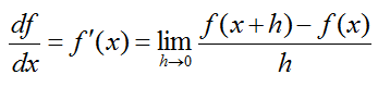
Figure 1. The definition of the derivative. The derivative f'(x) is the limit of the difference quotient as the step h goes to 0.

One good way to figure out practical meaning of a mathematical concept is to represent it in graphical form as much as possible. Fortunately most of calculus concept for single variable can be represented in a form of graph or illustration.

First let's look at the following illustration that shows the meaning of each component of the expression. I don't think I need any further explanation and hope you can figure out the meaning of this illustration just by looking at it. If this is the first time you saw this kind of illustration, I would recommend you to copy this illustration and all the mathematical expression and arrows by hand. (If you want to create this kind of graph for other functions that you want try "Matlab/Octave Code I" appended at the end).

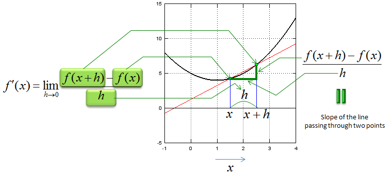
Figure 2. The difference quotient is the slope of the line through two points on the curve. With h = 1 this line is a secant, not yet the tangent.

• The black curve is f(x) = x(x - 2) + 5 : this is the function in Matlab/Octave Code I, which is x² - 2x + 5. Its minimum is at x = 1, where f(1) = 4.
• The two points are x = 1.5 and x + h = 2.5 : so h = 1. The function values are f(1.5) = 4.25 and f(2.5) = 6.25.
• The green step shows the two differences : the horizontal leg is h, and the vertical leg is f(x+h) - f(x) = 2. Their ratio, 2/1 = 2, is the slope of the red line.
• The red line is only an approximation : the true derivative is f'(x) = 2x - 2, so f'(1.5) = 1. The secant slope 2 is twice that value, because h = 1 is far from 0.

So the picture gives you every part of the expression except the limit. The fraction is the slope of a line through two points, and that slope depends on how far apart you put the points. Let's now see what the limit does to this line.

• A difference quotient is a secant slope : it is the change in f(x) divided by the change in x, over a finite step h.
• A large step gives a wrong slope : for x² - 2x + 5 at x = 1.5, h = 1 gives 2 while the derivative is 1.

What happens when h gets closer to 0 ?

Now let's think of the meaning of "limit" in this expression. It says "h approaches to 0". It means "it get closer to 0". What would the graph look like when h gets closer to 0. You would get the meaning of this mathematical expression at the last graph shown below. (If you want to create this kind of graph for other functions that you want try "Matlab/Octave Code II" appended at the end).

The plots below use the same curve, but the first point is now fixed at x = 2. The panels run in rows, from left to right and then from top to bottom. In each panel h is a little smaller, from about 1.41 in the first panel down to 0.0001 in the last one.

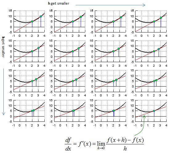
Figure 3. As h gets smaller, the second point slides along the curve toward the first one, and the secant line turns into the tangent line at x = 2.

For this function you can compute the secant slope exactly. With x = 2, f(2 + h) - f(2) = 2h + h², so the secant slope is 2 + h. It is always larger than 2 by exactly h, and it goes to 2 as h goes to 0. The derivative formula gives the same value, because f'(2) = 2*2 - 2 = 2. The table below lists a few of the panels.

Now let's look at the mathematical expressions for 'differentiation' again. I hope this make more sense to you by now.

Figure 4. The derivative is the change in f(x) divided by the change in x, in the limit of a very small change in x.

This is also where the notation df/dx comes from. The letter d stands for a very small change, so df/dx reads as a small change in f divided by the small change in x that caused it. A computer cannot take the limit. It stops at a small h, as in the last panel of Figure 3. The Numerical Differentiation page shows the forward and backward versions of this approximation.

• The limit turns a secant into a tangent : the derivative is the slope of the tangent line at one point.
• The error of the secant shrinks with h : for x² - 2x + 5 at x = 2 the secant slope is exactly 2 + h.
• A numerical derivative is a secant with a small h : h = 0.0001 already gives 2.0001 here.

How does differentiation extend to a function of two variables ?

A surface has a different slope in every direction you move on it. So a function of two variables does not have one single derivative at a point. Instead, we take the derivative along each axis separately, and each of these is called a partial derivative.

What if we extend this concept to two variable function ? Mathematical expression for multivariable differentiation looks as follows.

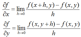
Figure 5. Partial derivatives. Only one variable moves by h, and the other one is held fixed.

Each line of Figure 5 is the single variable definition again. For the partial derivative with respect to x, y is held at a fixed value, and only x moves by h. So you take a slice of the surface along the x direction and find the slope of that slice. The partial derivative with respect to y does the same along the y direction.

It is not always easy to represent this multi variable differentiation in graphical form, but I picked a function so that I can graph it. It looks as shown below.  (If you want to create this kind of graph for other functions that you want try "Matlab/Octave Code III" appended at the end. You should be a little bit careful about changing equations in the code. You should change the equations for three lines, lines for fxy, Zx, Zy. I admit that my code is not so wisely written. This is why you have to change the equation in multiple locations).

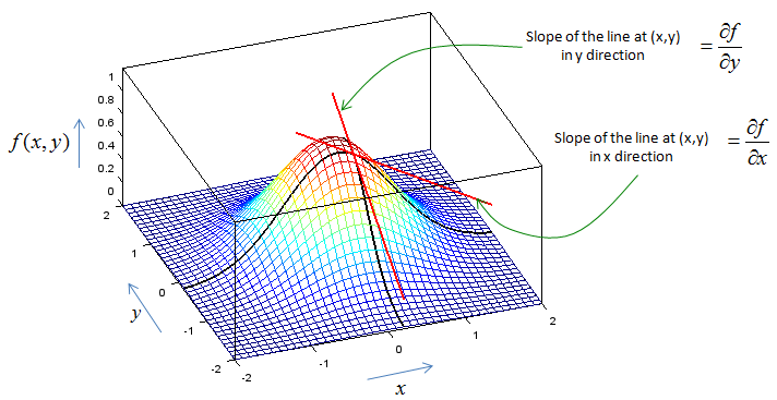
Figure 6. The surface f(x,y) = e^{-(x2 + y2)} with two slices through one point. Each red line is the tangent of one slice, and its slope is one partial derivative.

• The surface is a two variable Gaussian : Code III defines fxy as exp(-(x.^2+y.^2)). Its peak value is 1, at x = 0 and y = 0.
• The point is x = 0.2 and y = -0.2 : these are x0 and y0 in the code. The function value there is e^-0.08 = 0.923.
• The two black curves are the slices : one runs along x with y fixed at -0.2, and the other runs along y with x fixed at 0.2.
• The slopes have equal size and opposite sign : the partial derivatives are -2x f(x,y) and -2y f(x,y). At this point they are -0.369 in the x direction and +0.369 in the y direction. The signs differ because x0 is positive and y0 is negative. A step in +x moves away from the peak, and a step in +y moves toward it.

The two partial derivatives together form the gradient of f. The gradient points in the direction where the surface rises fastest, and its length is that rate of rise. At the peak, both partial derivatives are 0, so the gradient is 0 there. The Gradient page continues from here.

If you don't have any problem with what I described above and it is too simple for you, check if you can still understand the meaning of the differentiation when the function is a complex variable function or vector function. I would not come back this topic right away, but in real engineering you would see more of the case for complex function or vector functions. (I will come back to this topic, when I complete all the basic pages).

• A partial derivative is an ordinary derivative along one axis : all the other variables are held fixed.
• Two variables give two slopes at every point : together they form the gradient.
• A zero gradient marks a flat point : the peak of the Gaussian has both partial derivatives equal to 0.

How can you draw these graphs in Matlab or Octave ?

The three listings below produced Figure 2, Figure 3 and Figure 6. Each one approximates a derivative the same way the definition does: it picks two points, computes the slope between them, and draws the line with that slope. Change the function and the points to see the same pictures for another curve.

One warning before you run them. The listings use the operators .- and .+, as in x .- 2. These are Octave syntax, and MATLAB does not accept them. In MATLAB, write - and + instead. They give the same result in Octave too, because subtraction and addition are always element by element.

Matlab/Octave Code I

This listing draws Figure 2. It computes the slope a and the intercept b of the line through the points x1 = 1.5 and x2 = 2.5, and then plots the curve, the line and the two points.

xmin = -1;

xmax = 4;

ymin = -5;

ymax = 15;

 

x = xmin:0.1:xmax;

 

fx = @(x)[x .* (x .- 2) + 5];

 

x1 = 1.5;

y1 = fx(x1);

x2 = 2.5;

y2 = fx(x2);

 

a = (y1-y2)/(x1-x2);

b = (x1*y2-x2*y1)/(x1-x2);

yd = a .* x + b;

 

hold on;

plot(x,fx(x),'k-','Linewidth',2);axis([xmin xmax ymin ymax]);

plot(x,yd,'r-');axis([xmin xmax ymin ymax]);

stem([x1 x2],[y1 y2],'MarkerFaceColor',[0 1 0]);

grid;

hold off;

Matlab/Octave Code II

This listing draws Figure 3. It fixes x1 = 2.0 and runs a loop of 16 panels. In panel i, the second point is x1 + hmax - i*hstep + 0.0001, so h goes from about 1.41 down to 0.0001. The small 0.0001 keeps the last h from being exactly 0, which would make the slope 0/0.

xmin = -1;

xmax = 4;

ymin = -5;

ymax = 15;

 

x = xmin:0.1:xmax;

 

fx = @(x)[x .* (x .- 2) + 5];

 

x1 = 2.0;

y1 = fx(x1);

hmax = 1.5;

hstep = hmax/16;

 

for i = 1:16,

 

x2 = x1 + hmax - i*hstep + 0.0001;

y2 = fx(x2);

 

a = (y1-y2)/(x1-x2);

b = (x1*y2-x2*y1)/(x1-x2);

yd = a .* x + b;

 

subplot(4,4,i);

 

hold on;

plot(x,fx(x),'k-','Linewidth',2);axis([xmin xmax ymin ymax]);

plot(x,yd,'r-');axis([xmin xmax ymin ymax]);

stem([x1 x2],[y1 y2],'MarkerFaceColor',[0 1 0]);

grid;

hold off;

 

end;

Matlab/Octave Code III

This listing draws Figure 6. It builds the surface with meshgrid, takes the slices Zx and Zy through the point x0 = 0.2 and y0 = -0.2, and computes each slope from two points only 0.00001 apart. The comment says slot, but it means slope.

 

xmin = -2;

xmax = 2;

ymin = -2;

ymax = 2;

 

x0 = 0.2;

x1 = 0.20001;

y0 = -0.2;

y1 = -0.20001;

 

x = xmin:0.1:xmax;

y = ymin:0.1:ymax;

[X,Y] = meshgrid(x,y);

 

fxy = @(x,y)[exp(-(x.^2+y.^2))];

Z = fxy(X,Y);

 

Zx = exp(-(x.^2+y0.^2));

Zy = exp(-(x0.^2+y.^2));

 

zx0 = fxy(x0,y0);

zx1 = fxy(x1,y0);

 

a = (zx0-zx1)/(x0-x1);

b = (x0*zx1-x1*zx0)/(x0-x1);

Zxd = a .* x + b;

 

zy0 = fxy(x0,y0);

zy1 = fxy(x0,y1);

 

a = (zy0-zy1)/(y0-y1);

b = (y0*zy1-y1*zy0)/(y0-y1);

Zyd = a .* y + b;

 

hold on;

mesh(X,Y,Z);

plot3(x,y .* 0 .+ y0, Zx, 'linewidth',2,'color','k');axis([-2 2 -2 2 0 1.2]);

plot3(x .* 0 .+ x0,y, Zy, 'linewidth',2,'color','k');axis([-2 2 -2 2 0 1.2]);

plot3(x,y .* 0 .+ y0, Zxd, 'linewidth',2,'color','r');axis([-2 2 -2 2 0 1.2]); % slot at x0,y0 in x direction

plot3(x .* 0 .+ x0,y, Zyd, 'linewidth',2,'color','r');axis([-2 2 -2 2 0 1.2]); % slot at x0,y0 in y direction

view(-20,50);

hold off;

The two point slope in these listings has an error that shrinks with the distance between the points. Code I uses a distance of 1 and shows that error clearly. Code III uses 0.00001, so its red lines are practically the tangent lines.

• All three listings use the same two point slope : a = (y1-y2)/(x1-x2) is the difference quotient of Figure 1.
• Replace .- and .+ for MATLAB : plain - and + work in both MATLAB and Octave.