Numerical differentiation estimates a derivative from function values at a few nearby points. We need it whenever the function is known only as a table of samples, such as a measured signal or the output of a simulation. The idea is to replace the limit in the definition of the derivative with a small but finite step h. This page shows the three first order difference formulas. Then it builds the second order formula and writes it as a matrix, so that one matrix product differentiates a whole table at once. The last section measures how accurate each formula is.

The topics on this page are listed below.

• First Order Differentiation
• Second Order Differentiation
• How accurate are the difference formulas ?

First Order Differentiation

The derivative f^'(x) is the slope of the tangent line at x. With only samples of f, we cannot draw the tangent line. But we can draw a straight line through two samples and take its slope. The three formulas below differ only in which two samples they use.

Backward Differentiation

The backward formula uses the current point and the point one step before it. It needs no future sample, so it works on data that arrives in real time.

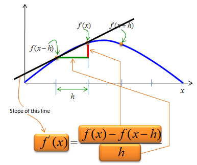
In the picture above, the green line is the step h and the red line is the change f(x) - f(x-h). The black line passes through f(x-h) and f(x), and its slope is the estimate f^'(x) = (f(x) - f(x-h)) / h. On this curve the black line is steeper than the true tangent at x, because the curve bends down between the two points.

Forward Differentiation

The forward formula uses the current point and the point one step after it. It is the formula closest to the textbook definition of the derivative, with the limit removed.

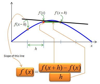
Here the black line passes through f(x) and f(x+h), and the estimate is f^'(x) = (f(x+h) - f(x)) / h. On this curve the line is flatter than the true tangent at x. So the forward and backward estimates err in opposite directions for the same curve.

Centered Differentiation

The centered formula uses the points one step before and one step after x, and it skips f(x) itself. The two opposite errors of the forward and backward formulas then cancel to a large extent.

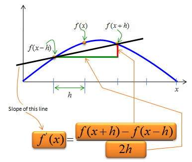
The black line passes through f(x-h) and f(x+h), so it spans 2h, and the estimate is f^'(x) = (f(x+h) - f(x-h)) / 2h. The centered estimate is the average of the forward and backward estimates. For the same h it is usually much more accurate, as the last section shows with numbers.

• All three formulas take the slope of a line through two samples : they differ only in where the two samples sit relative to x.
• Backward and forward errors have opposite signs : on a curve that bends down, the backward line is too steep and the forward line is too flat.
• The centered formula is the average of the other two : the opposite errors cancel, so it is the usual choice when samples on both sides are available.

Second Order Differentiation

The second derivative needs three samples, because it measures how the slope itself changes. Applying the forward and backward formulas one after the other gives the standard three point formula. Writing that formula as a row vector then turns the differentiation of a whole table into one matrix product.

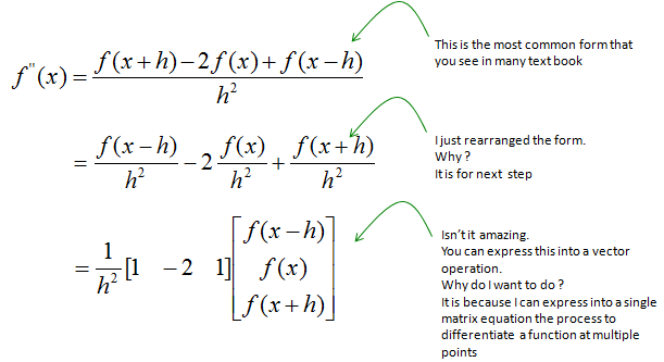
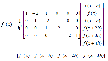
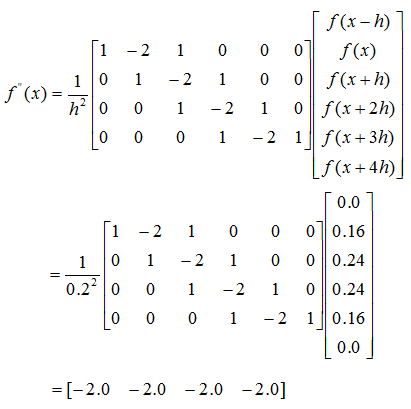
The upper picture of the two above starts from f^''(x) = (f(x+h) - 2f(x) + f(x-h)) / h². This is the forward difference minus the backward difference, divided once more by h: ((f(x+h) - f(x))/h - (f(x) - f(x-h))/h) / h. The weights 1, -2 and 1 are then collected into the row vector [1 -2 1]. The lower picture shifts that row one column to the right for each new point. So a 4 x 6 matrix times six samples gives the second derivative at four points. Each row loses one sample on each side, so n samples give n - 2 derivatives.

Example 1

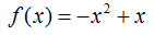
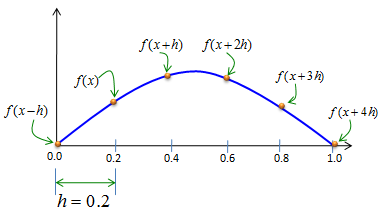
The first example uses a parabola, because its second derivative is known exactly. That makes it a clean test of the matrix formula. The step size is h = 0.2, and the six samples run from x = 0 to x = 1.

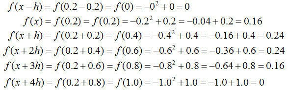
If you are not confident on the calculation, click here to get the excel spreadsheet that I made.

The result is -2.0 at all four points, and the exact second derivative of -x² + x is also -2. The match is exact, not approximate. The three point formula has an error proportional to h² times the fourth derivative of f. For a parabola the fourth derivative is 0, so the formula makes no error for any h.

Example 2

The second example uses f(x) = cos(x), whose exact second derivative is -cos(x). The linked spreadsheet samples it with h = 0.2 from x = 0 to 6.4, which gives 33 samples. So the matrix has 31 rows and 33 columns, which is too large to write out here.

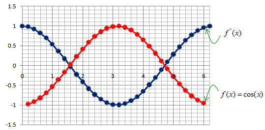
Since this matrix is too large, it would be difficult to calculate manually. So I implemented this in Excel and you can get the spreadsheet here.

In the plot above, the blue curve starts at 1 at x = 0, so it is cos(x). The red curve starts at about -1 at x = 0.2, so it is the numerical f^''(x). It has no point at x = 0, because the matrix needs one sample on each side of every point. The two labels on the right point the other way around: the label f^''(x) points at the blue curve and the label f(x) = cos(x) points at the red curve. Read the curves by their starting values instead. The red curve is the mirror image of the blue one, which is what -cos(x) should be. With h = 0.2 the formula returns -cos(x) times 0.9967, so the error is about 0.33 percent and too small to see in the plot.

• The second derivative formula uses the weights 1, -2 and 1 : it is a difference of two first differences, divided by h².
• A banded matrix differentiates a whole table : each row holds 1, -2, 1, shifted by one column, and n samples give n - 2 results.
• The formula is exact for a parabola : its error depends on the fourth derivative, which is 0 for any polynomial of degree 3 or less.

How accurate are the difference formulas ?

Every formula on this page replaces a limit with a finite step, so every one of them makes an error. We want to know how the error depends on h. The answer decides which formula to use and how small h should be.

The Taylor series gives the answer. Expanding f(x+h) around x gives f(x) + h f^'(x) + (h²/2) f^''(x) + (h³/6) f^'''(x) + ... . Put this into the forward formula, and the first error term is (h/2) f^''(x). So the forward error is proportional to h, and the backward error is the same with the opposite sign. In the centered formula the h² terms of f(x+h) and f(x-h) cancel. Its first error term is (h²/6) f^'''(x), so the error is proportional to h². The three point second derivative formula also has an error proportional to h², namely (h²/12) times the fourth derivative.

Let's test this on f(x) = sin(x) at x = 1. The exact first derivative is cos(1) = 0.540302, and the exact second derivative is -sin(1) = -0.841471.

The table confirms the Taylor analysis. When h drops by a factor of 10, the forward and backward errors drop by a factor of 10. The centered and second derivative errors drop by a factor of 100. The forward and backward errors also have opposite signs, as the sketches in the first section suggest.

A smaller h is not always better on a computer. The numerator is a difference of two nearly equal numbers, so floating point round-off error grows as h shrinks. In double precision, the forward error for this example is about 4.2 x 10^-7 at h = 10^-6 and about 3.0 x 10^-9 at h = 10^-8. At h = 10^-10 it grows again, to about 5.8 x 10^-8, instead of falling further. For the centered formula, the smallest error among the steps 10^-4, 10^-6, 10^-8 and 10^-10 is about 3 x 10^-11, at h = 10^-6. With measured data, noise plays the same role as round-off, and it usually sets a much larger lower limit on h.

• Forward and backward formulas are first order accurate : their error is proportional to h.
• The centered and three point formulas are second order accurate : their error is proportional to h², so a 10 times smaller h gives a 100 times smaller error.
• Round-off sets a lower limit on h : below about 10^-8 for the forward formula in double precision, a smaller h makes the result worse.