Divergence answers one question about a vector field: at a given point, does the field spread out, gather in, or neither? The answer is a single signed number. A positive value marks a source, a negative value marks a sink, and zero means that as much flows in as flows out. This page starts from the verbal description, then takes the two variable definition apart piece by piece. After that it works through five example fields. Finally it shows how divergence connects to the flux through a closed boundary.

The topics on this page are listed below.

• What does divergence measure ?
• How is divergence calculated ?
• Examples
• How does divergence connect to the flux through a boundary ?

What does divergence measure ?

Let's first agree on what we want to measure, before any formula. Picture the arrows of a vector field around one point. We want one number that says whether those arrows carry more out of the point than into it.

Divergence is a mathematical tool (a vector operator) to indicate whether field vectors from a specific point is spreading out of the point or merge into the point.

It is hard to explain verbably, so everybody explain the concept a little bit different ways. If I give you another example of description of Divergence from WiKi(http://en.wikipedia.org/wiki/Divergence), it goes as follows.

In vector calculus, divergence is a vector operator that measures the magnitude of a vector field's source or sink at a given point, in terms of a signed scalar. More technically, the divergence represents the volume density of the outward flux of a vector field from an infinitesimal volume around a given point.

I think this is better than my description, but still is a little vague. Everybody would want somebody to explain a difficult concept without using math, but eventually you would realize that it is impossible to have 'clear and solid' understanding without directly tackling the math. I think the best way is to get the overall picture with picture / diagram / illustration and verbal description and then look into the mathematical definition. When you start look into the mathematical definition, you have to analyze every component of definition in very detailed level. Without this kind of detailed analysis, you may get the mathematical solution of it but would not have 'practical understanding' (real meaning) of the solution.

The quoted description has two key words. The first is "signed scalar". Divergence is a number with a sign, not an arrow. The second is "outward flux from an infinitesimal volume". Draw a tiny box around the point, add up the flow out through its walls, and divide by the size of the box. The limit of this ratio, as the box shrinks, is the divergence. The next section shows that the partial derivatives in the definition compute exactly this ratio.

• Divergence is a signed number at each point : positive means a source, negative means a sink, and zero means balanced flow.
• It is a density of outward flux : it measures net outflow per unit area in two dimensions, or per unit volume in three.
• It describes one point, not the whole field : the same field can have sources in one place and sinks in another.

How is divergence calculated ?

The verbal picture needs a formula before we can compute anything. The formula is short, but each term has a specific meaning. So we take it apart on a magnified piece of a vector field.

Now let's look at the mathematical definition of Divergence. It is defined as follows (this is the definition when the number of variable is two. You can expand this to N variables. I used two variable function because it is easier to show in picture).

First you would notice that the result of Divergence is 'Scalar'. Another thing you have to notice is that P and Q are the two components of a vector function F, not a scalar function.

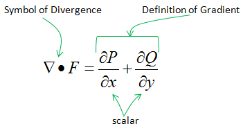
The picture above shows the symbol ∇ ⋅ F and the sum ∂P/∂x + ∂Q/∂y, and it marks both partial derivatives as scalars. The label at the top right says "Definition of Gradient", but the formula under it is the definition of divergence. The gradient is a different operator, which you can find on the Gradient page.

Now let's analyze each component of this mathematical equations. In following example, I cut a small section of a vector field and magnify it as shown on the right side. I just focused two vectors. First, make it sure that you understand the meaning of each of these lines (green lines and red lines) and vectors (blue arrows). Green line indicate the x component of the vectors and Red line indicates the y component of the vector.

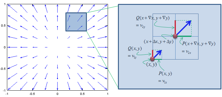
In the magnified box, the lower vector sits at (x, y) and has the components P(x,y) = v_1x and Q(x,y) = v_1y. The upper vector sits at (x + Δx, y + Δy) and has the components v_2x and v_2y. Some labels in the picture write ∇x and ∇y where Δx and Δy are meant. Both mean the small step between the two points, not the gradient operator.

Now let's compare how much the x components of the two vectors (Green Lines) changed and how much the y components of the two vectors changed. Divergence is the sumation of these two changes (change in the x direction and change in the y direction). In other word, divergence is the 'net changes of the two vectors' as shown below.

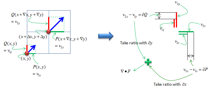
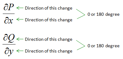
The two pictures above complete the calculation. The change of the x component, v_2x - v_1x, is divided by the step in x. The change of the y component, v_2y - v_1y, is divided by the step in y. The sum of the two ratios is the divergence. The picture directly above points out that each ratio compares changes along the same axis, 0 or 180 degrees apart. So only the part of P that changes along x counts, and only the part of Q that changes along y counts.

If the net change (Divergence) is plus value, you would see /feel that something is expanding from the observation point (in this example, the observation point is (x,y)). If the net change (Divergence) is minus(negative) value, you would see /feel that something is shriking into the observation point (in this example, the observation point is (x,y)).

One confusing point is the case when 'Divergence(net change)' is 0. There are two case when divergence is 0. One is the case when there is no change at all, meaning no change in x direction, no change in y direction. This is obvious. You would not feel any changes at the observation point.

However, there is another case where you will have 'Divergence 0' (0 Net change). It is the case when both x component of the vector and y component of the vector changes and the amount of the change is same, but the direction of change is opposite. For example, if the vector expanded 2 times in positive direction on x axis and expanded 2 times in negative direction on y axis, the net change (divergence) becomes 0.

A field that shows this second case is P = x, Q = -y. The x component grows by 1 per unit step in x, and the y component shrinks by 1 per unit step in y. So ∇ ⋅ F = 1 - 1 = 0. The flow is not at rest. It comes in along the y axis and leaves along the x axis at the same rate.

In three dimensions one more term joins the sum, ∇ ⋅ F = ∂P/∂x + ∂Q/∂y + ∂R/∂z, where R is the z component. Each term still compares the change of one component along its own axis.

• Each term compares a component with its own axis : ∂P/∂x uses the x component along x, and ∂Q/∂y uses the y component along y.
• The sum decides the sign : a growing x component can be cancelled by a shrinking y component, and then the divergence is 0.
• Zero divergence does not mean a still field : the field P = x, Q = -y moves everywhere except at the origin, and its divergence is 0.

Examples

Each example below gives a field, its plot with a few marked points, and the calculated divergence. Try to guess the sign at each marked point from the plot first. Then check the guess against the formula.

Example 1

The first field grows in proportion to the distance from the origin, and every arrow points outward. It is the same field that the Vector Field page uses to show how a field is drawn.

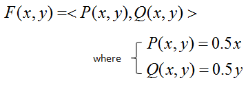
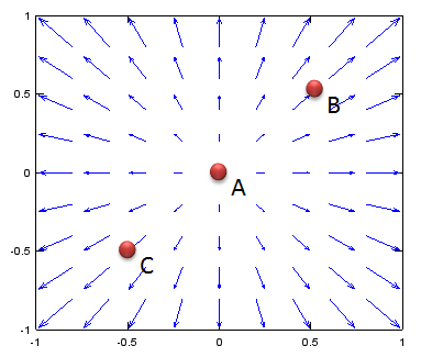
The divergence is 1 at every point, so A, B and C all have the same value. This can be a surprise at A, where the arrow has zero length. The divergence does not depend on the length of the arrow at the point. It depends on how the arrows change around the point, and here they grow at the same rate everywhere.

Example 2

The second field is uniform. Every arrow has the same length and points in the same direction, to the right. This example shows that a strong flow does not by itself mean a large divergence.

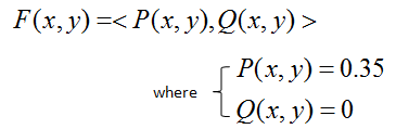
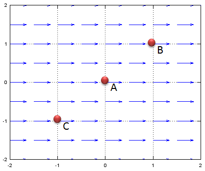
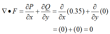
The divergence is 0 at A, B and C. Everything that flows into a small box on its left side flows out on its right side. So nothing is gained or lost inside the box.

Example 3

The third field has only an x component, and its length follows a sine wave along x. So the divergence changes from place to place. This example shows positive, zero and negative divergence in one field.

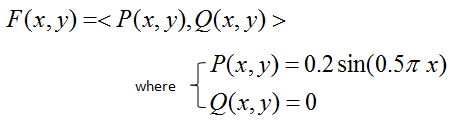
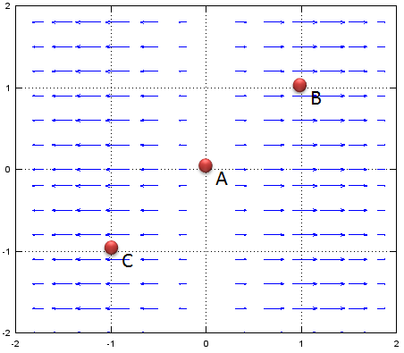
At A, where x = 0, the divergence is 0.1π, about 0.314. The arrows point away from the vertical line x = 0 on both sides, so A is on a line of sources. At B and C, where x = 1 and x = -1, the cosine is 0, so the divergence is 0. These are the places where the arrows are the longest, but they are not changing length there. Near the left and right edges, at x = +/-2, the divergence reaches -0.314. There the arrows from both sides meet, and the field acts as a sink.

Example 4

The fourth field mixes x and y in its components. Its divergence depends on y only, which you cannot easily guess from the plot. This example has five marked points, labelled A to E.

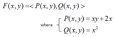
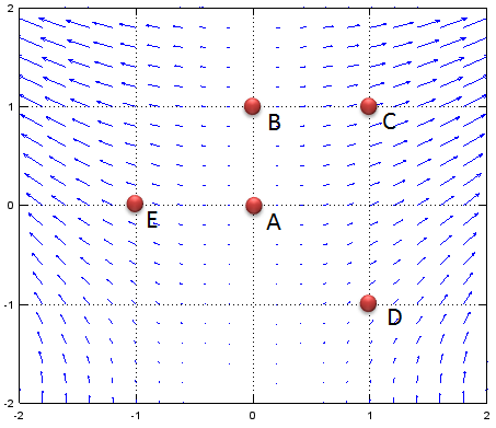
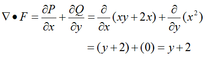
The divergence is y + 2, so it depends only on the height of the point. At A (0, 0) and E (-1, 0) it is 2. At B (0, 1) and C (1, 1) it is 3. At D (1, -1) it is 1. All five points are sources, and the source gets stronger as y grows. The divergence reaches 0 on the line y = -2, the bottom edge of the plot, and would be negative below it.

Example 5

The fifth field is a rotation. The arrows go around the origin in a clockwise direction, and none of them points toward or away from the origin. This example shows the case where a clearly moving field has no divergence.

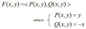
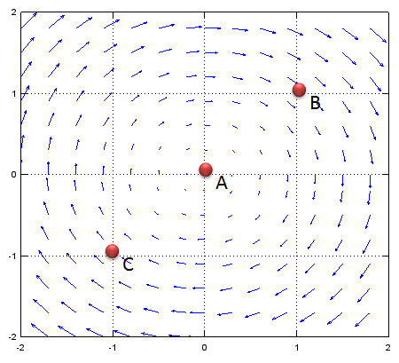
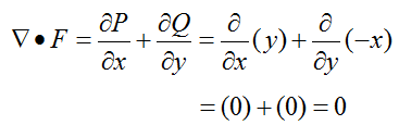
The divergence is 0 at A, B and C. The field only turns, so every small box has as much flow in as out. The curl measures this turning instead, and for this field the curl is -2 everywhere.

• The length of the arrow at a point does not decide the divergence : Example 1 has divergence 1 at the origin, where the arrow is zero, and Example 2 has divergence 0 with long arrows.
• Divergence can change sign within one field : in Example 3 it is 0.314 at x = 0 and -0.314 at x = +/-2.
• A rotation has zero divergence : Example 5 moves everywhere except at the origin, but nothing spreads or gathers.

How does divergence connect to the flux through a boundary ?

Divergence is defined at a point, but we often need the total outflow through a closed boundary. The divergence theorem connects the two. It says that adding up the divergence over a region gives the flux through the boundary of that region.

In two dimensions the theorem reads ∫∫ ∇ ⋅ F dA = ∮ F ⋅ n ds. The left side adds the divergence over the region. The right side adds the outward normal component of F along the boundary curve, where n is the outward unit normal. The reason is simple. Each small box inside the region shares its walls with its neighbours. The flow out of one box through a shared wall is the flow into the next box, so these terms cancel. Only the walls on the outer boundary are left.

Let's check this with Example 1 and a unit circle. The divergence is 1, and the area of the circle is π, so the left side is π. On the circle, F = 0.5 (x, y) points straight outward with length 0.5. So F ⋅ n = 0.5 everywhere on the boundary, and the right side is 0.5 x 2π = π. Both sides agree.

Example 4 gives a less symmetric check on the unit square from (0, 0) to (1, 1). The left side is the integral of y + 2 over the square, which is 2.5. On the right side we add the outward flow through the four edges. The right edge, at x = 1, has P = y + 2, and it contributes 2.5. The left edge, at x = 0, has P = 0, and it contributes 0. The top edge contributes the integral of Q = x², which is 1/3. The bottom edge contributes -1/3, because the outward normal there points down. The total is again 2.5.

In three dimensions the same theorem connects a volume integral with a surface integral. Gauss Law for the electric field is one form of it. The divergence of the electric field is the charge density divided by ε₀. So the flux through a closed surface is the enclosed charge divided by ε₀.

• The divergence theorem adds point values into a boundary total : the integral of the divergence over a region equals the outward flux through its boundary.
• Inner walls cancel : the flow between neighbouring small boxes appears once as outflow and once as inflow.
• Both examples check out : Example 1 gives π on the unit circle, and Example 4 gives 2.5 on the unit square, from either side of the theorem.