Gradient

The gradient turns a function of several variables into a vector at every point. That vector answers a practical question: if you stand at this point, which way is uphill, and how steep is it? The answer is used everywhere, from the electric field, which is minus the gradient of the potential, to gradient descent in machine learning. This page builds the gradient from its two partial derivatives. It shows how the vector changes when one slope is larger than the other. It also explains why the gradient always crosses the contour lines at a right angle.

The topics on this page are listed below.

How is the gradient defined ?

Let's start with the formula and read each symbol in it. The definition is short. But it mixes scalars and vectors, and the reader has to keep track of which is which.

Mathematical Definition of Gradient (2 variable case) is as follows. The practical meaning of the gradient is "a vector representing the direction of the steepest upward path at specified point". Do you understand how the following mathematical expression represent the steepest path ? If you understand this, you don't have to read this page any more.

As you see from the mathematical definition, gradien is a vector meaning that it has a magnitude and direction and you have to understand what the magnitude indicate and what the direction indicate.

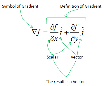
Definition of the gradient of a two variable function

The picture above labels the parts of the definition.

The symbol ∇f, read "del f" or "grad f", is the gradient of the function f.
The partial derivatives ∂f/∂x and ∂f/∂y are scalars. Each one is the slope of the surface in one direction.
The unit vectors i and j are vectors. They carry the directions of the x axis and the y axis.
Each scalar multiplies one unit vector, and the sum of the two products is a vector. So the gradient of a scalar function is a vector.

The same definition extends to more variables. For a function f(x, y, z), the gradient is ∇f = (∂f/∂x) i + (∂f/∂y) j + (∂f/∂z) k, and in general there is one component for each variable. The operator ∇ also appears in the divergence ∇ ⋅ F and in the curl. There it acts on a vector field instead of a scalar function.

The gradient turns a scalar function into a vector : each partial derivative becomes the component along its own axis.
The gradient points in the direction of steepest increase : the direction of steepest decrease is -∇f, which is the one used by gradient descent.
The length of the gradient is the steepest slope : no other direction at that point gives a larger rate of change.

How do the two partial derivatives build the gradient vector ?

The formula says to add two vectors. The pictures in this section show what those two vectors look like on a real surface. They also show how the sum changes when one slope is larger than the other.

Let's suppose you have a function (two variables) as shown below (left side). Now take one rectangular segment of the surface and magnify it as shown on the right side. Now draw the vectors represented by vector i and j. The vector i is in line with red vector and j is in line with blue vector in this example. i and j vector are unit vectors meaning that their magnitude are 1. The real size of the red vector is determined by the slope of the side of surface segment(green rectangle) in x direction and the real size of the blue vector is determined by the slope of the side of surface segment(green rectangle) in y direction. Make it sure that you clearly understand this (the meaning of the illustration on top right.)

Now you have the two vectors marked in blue and red (again make it sure that you know the meaning of the blue and red vector). If you sum up the two vectors, you will have another vector marked in a green vector. That is the gradient at the point. Do you understand now how you get the blue and red vector and what they mean, and how you get the green vector and what it mean ?

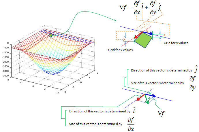
Gradient vector on a magnified segment of a bowl shaped surface

The picture above has three parts.

On the left is a bowl shaped surface. Its value is 0 near the rim and drops to about -3500 at the centre. One small green segment near the rim is marked.
At the upper right, the segment is magnified. The red arrow runs along the grid line for x values, and the blue arrow runs along the grid line for y values. Dashed arrows connect each one to its term in the formula.
At the lower right, the labels explain the arrows. The direction of the red arrow comes from i, and its size comes from ∂f/∂x. The direction of the blue arrow comes from j, and its size comes from ∂f/∂y. The green arrow is their sum, ∇f.

Just by looking at the illustration shown above, you may think that the size of blue vector and red vector would always be similar and the green vector (gradient vector) would be about 45 degree angle from the two vectors. It is not true, the size of the blue and red vector and direction of green vector can vary widely depending on the value obtained by the differentials in each direction. Followings are some of the examples.

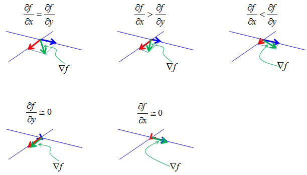
Gradient direction for five different ratios of the two partial derivatives

The five sketches above keep the same two axes and change only the two slopes.

When ∂f/∂x = ∂f/∂y, the red and blue arrows have the same length, and ∇f lies halfway between them.
When ∂f/∂x > ∂f/∂y, the red arrow is longer, and ∇f leans toward the x direction.
When ∂f/∂x < ∂f/∂y, the blue arrow is longer, and ∇f leans toward the y direction.
When ∂f/∂y is close to 0, the blue arrow almost disappears, and ∇f lies along the x direction.
When ∂f/∂x is close to 0, the red arrow almost disappears, and ∇f lies along the y direction.

In numbers, the angle of the gradient from the x direction is arctan((∂f/∂y) / (∂f/∂x)), and its length is √((∂f/∂x)² + (∂f/∂y)²). So the ratio of the two slopes sets the direction, and their combined size sets the length.

Each partial derivative is one side of a right triangle : the gradient is the hypotenuse, so its length is the square root of the sum of the squares.
The ratio of the slopes sets the direction : the gradient leans toward the axis with the larger partial derivative.
A zero partial derivative removes one component : the gradient then lies along the other axis.

Why is the gradient perpendicular to the contour line ?

A contour line connects points where the function has the same value. Moving along it, the function does not change at all. The gradient is the direction of fastest change, so the two directions should be as different as possible, and this section shows that they meet at a right angle.

If you calculate the gradient vector in many different points on the contour graph, you can show the slope at those points. The gradient vectors are always right angle to the tangential line on the countour curve.

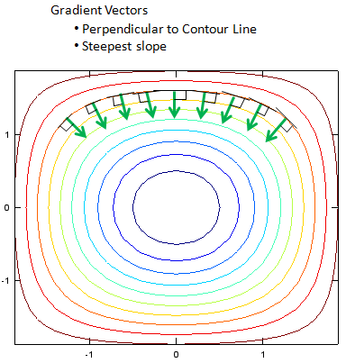
Gradient vectors crossing the contour lines at right angles

In the picture above, the green arrows sit on one contour line near the top. The small square marks at their feet show the right angle between each arrow and the contour line. The picture gives no contour values. If the centre is the lowest point, as in the bowl shaped surface above, the green arrows point downhill toward the centre. In that case they show -∇f, the direction of steepest descent. The gradient ∇f lies on the same lines and points the opposite way, outward and uphill. The right angle holds in both cases.

The reason for the right angle comes from the directional derivative. Take any unit vector u. The rate of change of f in the direction of u is D_uf = ∇f ⋅ u = |∇f| cos θ, where θ is the angle between ∇f and u. This value is largest when θ = 0, so the steepest increase is along ∇f, and its rate is |∇f|. The value is the most negative when θ = π, which is the direction -∇f. It is zero when θ = π/2. Along a contour line the function does not change, so the direction of the contour line must be the one with θ = π/2. That is, the contour line is perpendicular to the gradient.

The directional derivative is an inner product : D_uf = ∇f ⋅ u, so it depends on the angle between u and the gradient.
The gradient is normal to the contour line : the rate of change is zero along the contour line, and that happens only at a right angle to ∇f.
Steepest ascent and steepest descent lie on one line : ∇f goes uphill, -∇f goes downhill, and both cross the contour at a right angle.

How do you compute and use a gradient in practice ?

The pictures give the meaning, but a calculation makes it concrete. Let's take a simple bowl shaped function and check every statement above with numbers. The same numbers then show one step of gradient descent.

Take f(x, y) = x² + 2y². The partial derivatives are ∂f/∂x = 2x and ∂f/∂y = 4y, so ∇f = 2x i + 4y j. At the point (1, 1), the gradient is (2, 4).

The length is |∇f| = √(4 + 16) = √20, about 4.472. This is the steepest slope at (1, 1).
The direction of steepest increase is (1, 2)/√5. The y component is larger, because f grows twice as fast in y as in x.
For comparison, the slope along the diagonal direction (1, 1)/√2 is (2 + 4)/√2, about 4.243. This is less than 4.472, as the directional derivative predicts.
The contour line through (1, 1) is x² + 2y² = 3. Its tangent direction there is (2, -1), and (2, 4) ⋅ (2, -1) = 0. So the gradient is perpendicular to the contour line.

Gradient descent uses -∇f to walk toward a minimum. Each step is x_new = x - α ∇f(x), where α is the step size. With α = 0.1 and the start point (1, 1), the first step goes to (1 - 0.2, 1 - 0.4) = (0.8, 0.6). The function value drops from 3 to 0.64 + 0.72 = 1.36. The y coordinate moves more than the x coordinate, because the slope is steeper in y.

The electric field is another common use. The electric field is minus the gradient of the electric potential, E = -∇V. So the field points from high potential to low potential, and the field lines cross the equipotential lines at right angles. This is the same right angle as between the gradient and the contour lines above.

Compute the partial derivatives first : the gradient at any point is then a simple substitution.
No direction beats the gradient : at (1, 1) the gradient slope is 4.472, while the diagonal gives only 4.243.
Gradient descent follows -∇f : one step with α = 0.1 lowers f from 3 to 1.36 for this example.