A vector field attaches an arrow to every point of a plane or a space. The arrow can stand for the velocity of water, the force on a charge, or the direction in which a system will move next. This page starts from that physical picture and then shows how to draw a field from its two component functions P(x,y) and Q(x,y). After that it walks through a set of example fields. It also shows how divergence and curl sort them into sources, sinks and rotations. The last part uses a vector field to see the solution of a differential equation without solving it.

The topics on this page are listed below.

• What is a vector field ?
• How do you draw a vector field from P and Q ?
• Examples of Vector Field
• What do divergence and curl tell you about these examples ?
• Applications of Vector Field

What is a vector field ?

Let's begin with a flow that nobody can model in full detail. The question is how much we can still say about it, and the answer is the idea of a vector field. We give up the detail of each drop and keep one arrow per location.

Let's assume that you are asked o create a mathematical model for the water flow shown below. How easy/difficult you think it would be ? It would be almost impossible to make a accurate model which can explain very detailed movement (flow) of the water.

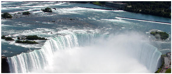
But you can come out with big picture of the overall flow without much difficulty. Here comes one way. Let's suppose you are on a small boat on the water(Don't try riding a boat or even fishing in this kind of dangerous place -:). The boat will float along the water flowing under the boat. Now you can measure the direction and the speed of the boat at a point and you can draw an arrow (vector) representing the direction and the speed. (The direction of arrow head would represent the direction that the boat is moving and the size of arrow would represent the speed of the boat). You can repeat this kind of measurement on many different point (the best way would be to make a fine grid lines and perform the measurement and draw a vector at each grid point), you would get a lot of arrows (vectors). And then you would see the overall pattern of the water flow as shown below. This is the concept of vector field.

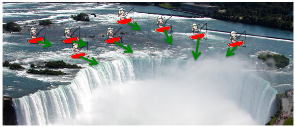
In the picture above, each boat carries one green arrow. Near the top of the picture the arrows point to the right and slightly down, along the river. Near the edge of the falls they turn down, toward the drop. No single arrow describes the river. Together, the arrows show where the water goes at every place, and that collection is the vector field.

Vector field is a method to represent 'degree of changes' in arrows (vectors) at many points along a specified line, surface or volumn.

• A vector field gives one arrow per point : the direction of the arrow is the direction of the flow there, and its length is the speed.
• The arrows are samples of a continuous field : we draw them on a grid, but the field has a value at every point between the grid points too.
• The pattern matters more than any single arrow : spreading, converging and turning are properties of many arrows together.

How do you draw a vector field from P and Q ?

The boat picture gives the idea, but a calculation needs a formula. In two dimensions a field is fully described by two functions, one for each component. Drawing the field is then a mechanical process that you repeat at every grid point.

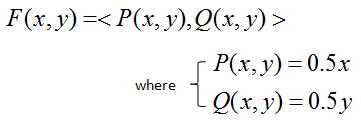
Now let's get into more mathematical context. In the above example, you 'felt' the flow with your body, now you are given a set of mathematical function as shown below. You see two functions P(x,y) and Q(x,y). Since this example is about the vectors on two dimensional plane, you have two variables x and y. P(x,y) is the function that gevern the vector component in x direction and Q(x,y) is the function that governs the vector component in y direction.

The way you draw a vector field is as follows. Pick any points in the coordinate. Plug the coordinate value into the function that represents the x component of a vector (P(x,y) in this example) and get the value, and draw a line on the x direction (green line in the following illustration). Next, Plug the coordinate value into the function that represents the y component of a vector (Q(x,y) in this example) and get the value, and draw a line on the y direction (red line in the following illustration). Following illustration shows this process for three different points. Make it sure that you understand this process very clearly and make some practice on your own. Otherwise, you would have difficulties interpreting the vector field.

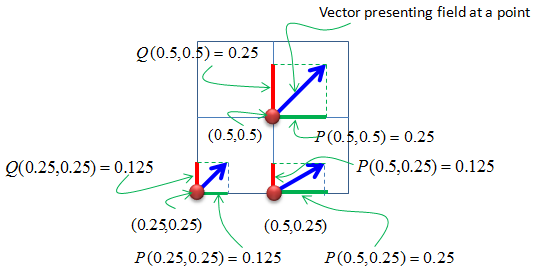
The picture above works through three points of the field P = 0.5x, Q = 0.5y.

• At (0.5, 0.5), P = 0.25 and Q = 0.25. The green and red lines have the same length, so the blue arrow points at 45 degrees.
• At (0.25, 0.25), P = 0.125 and Q = 0.125. The arrow has the same direction as before and half the length.
• At (0.5, 0.25), P = 0.25 and Q = 0.125. The label next to the red line of this point reads P(0.5,0.25) = 0.125, but it is the y component, so it should read Q(0.5,0.25) = 0.125.
• In every case the arrow points away from the origin, and its length grows with the distance from the origin.

If you repeat the process explained above for all the points on the grid, you will get a lot of arrows as shown below. This is called a vector field.

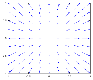
In the plot above, all arrows point away from the origin, and the arrows get longer toward the corners. This is what the formulas predict. The field is 0.5 times the position vector, so it points outward and grows in proportion to the distance. The arrow at the origin has zero length, which is why the centre of the plot is empty.

• P gives the x component and Q gives the y component : the arrow at (x, y) is the sum of a horizontal line of length P and a vertical line of length Q.
• Check a few arrows by hand : a plotting tool scales all arrows by one common factor, so only the relative lengths and the directions can be compared.
• The field 0.5 (x, y) spreads out from the origin : this is the simplest example of a source, and its divergence is 1 everywhere.

Examples of Vector Field

Reading a field from its formula is a skill that needs practice. The examples below go from simple straight line patterns to fields with two centres. Each one shows one typical shape: a saddle, a rotation, a source, a sink or a vortex.

In this section, I will try to give you as many examples as possible so that you can make practise of plotting vector field. (I will keep adding the examples) For every example, try to draw a couple of arrows by yourself and imagine the final outcome in your mind first and then check if it is the same as the plot given here.

Following is the matlab code to draw all the plots in this section. Of course, you have to change the equation for dx, dy in the code. I put various examples of the vector field plot in a slideshow format in my other notes here : www.freetechslide.com.

v = -1:0.2:1;  % you can change the range to best fit the plot
[x,y] = meshgrid(v);
dx=y;  % you can define P(x,y) part according to following examples. 
dy=-x - 0.25 .* y; % you can define Q(x,y) part according to following examples. 
quiver(x,y,dx,dy);
axis([-1 1 -1 1]); % you can change the range to best fit the plot

Before you run the code, note one detail. In the listing, dx and dy hold the values of P and Q at the grid points. They are not small steps, even though the names suggest it. The command quiver(x,y,dx,dy) draws the arrow (dx, dy) at the point (x, y), and it rescales all arrows together so that they fit the grid.

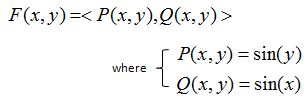
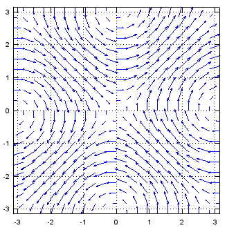
The first field is P = sin(y), Q = sin(x). The field is zero at every point where both x and y are multiples of π. Around the origin you see a saddle, where the flow comes in along one diagonal and leaves along the other. Around points such as (π, 0) the arrows turn in a circle instead.

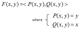
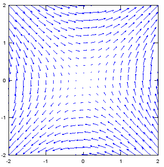
The next field is P = y, Q = x. It is a saddle again. Along the line y = x the arrows point away from the origin, and along the line y = -x they point toward it.

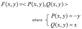
The field P = -y, Q = x is a pure rotation. Every arrow is at a right angle to the line from the origin, so the flow goes around the origin counterclockwise. The arrows get longer with the distance from the origin, like the points of a rotating wheel.

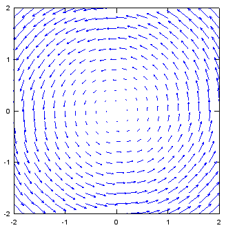
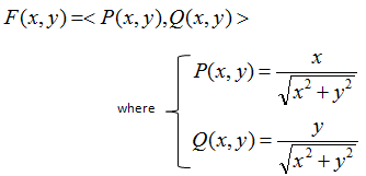
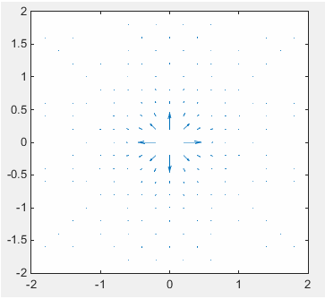
The next field divides the position vector by its own length, √(x² + y²). So every arrow has length 1 and points straight away from the origin. Compare it with the field 0.5x, 0.5y above. The directions are the same, but here the length no longer grows with the distance.

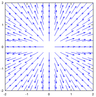
The next field is P = y / (x² + y²), Q = x / (x² + y²). The directions are the same as in the saddle P = y, Q = x. But the length falls as 1/r, where r is the distance from the origin. So the arrows are visible only close to the origin.

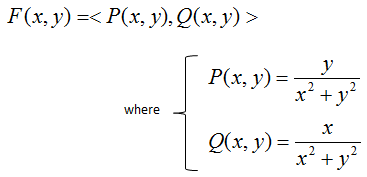
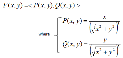
The next field points straight away from the origin, like the unit radial field. Its length falls as 1/r², which is the form of the electric field of a point charge. The arrows fade quickly, and only the ones next to the origin are clearly visible.

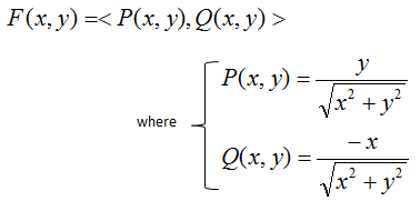
The field P = y / √(x² + y²), Q = -x / √(x² + y²) rotates clockwise, which is the opposite sense to the rotation above. Every arrow has length 1, so the pattern looks the same at every distance.

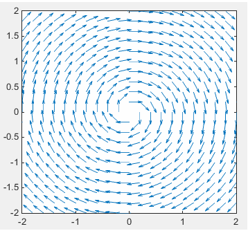
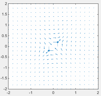
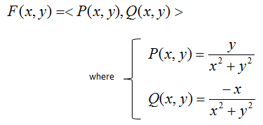
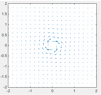
Dividing by x² + y² instead gives a vortex. The field still turns clockwise, but its length falls as 1/r. So the flow is fast near the centre and slow far away.

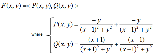
The remaining examples add two such terms, one centred at (-1, 0) and one centred at (1, 0). In this field both terms turn counterclockwise. Between the two centres the flows point in opposite directions, so they cancel near the origin.

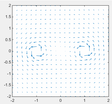
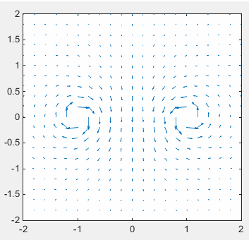
Here the vortex at (-1, 0) turns clockwise and the vortex at (1, 0) turns counterclockwise. Between the two centres the two flows now point the same way. So along the vertical line through the origin the field points straight down, and it is strongest at the origin.

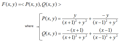
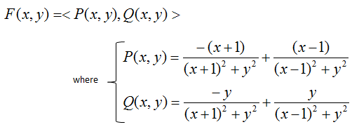
The next pair uses radial terms instead of rotating ones. The term at (-1, 0) points inward, which makes it a sink. The term at (1, 0) points outward, which makes it a source. The arrows between them run from the source to the sink.

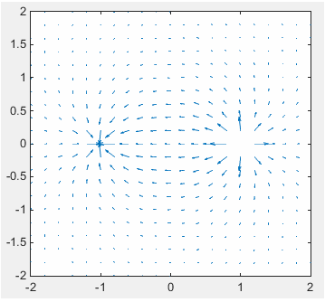
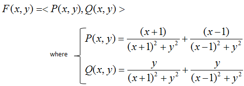
With two outward terms, both points are sources. Along the line between them, the two flows push against each other and cancel at the origin.

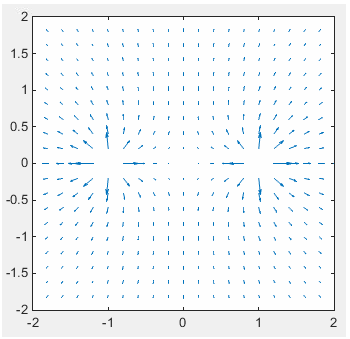
With two inward terms, both points are sinks. This field is the previous one with every arrow reversed.

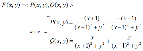
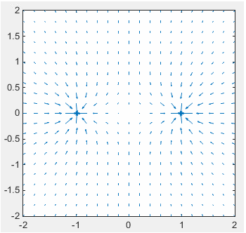
• Swapping or negating P and Q changes the pattern type : (x, y) spreads out, (y, x) makes a saddle, and (-y, x) rotates.
• The denominator sets how fast the field fades : dividing by r keeps the length at 1, dividing by r² gives a 1/r decay, and dividing by r³ gives a 1/r² decay.
• Fields with two centres are sums of two single fields : each term is centred at (-1, 0) or (1, 0), and the plot shows where the two terms reinforce or cancel.

What do divergence and curl tell you about these examples ?

Words such as source, sink and rotation describe the pictures. But we need numbers if we want to compare fields without plotting them. Divergence measures spreading, and curl measures turning, so these two operators give the numbers.

For a two dimensional field, the divergence is ∂P/∂x + ∂Q/∂y, and the curl is the single number ∂Q/∂x - ∂P/∂y. A positive curl means counterclockwise turning. The table below lists both values for the fields on this page. Here r is the distance from the origin, and each value holds away from the points where the field is not defined.

Some rows in the table look wrong at first. The vortex y/r², -x/r² clearly turns around the origin, yet its curl is 0. The two sources clearly push fluid outward, yet their divergence is 0. The reason is that curl and divergence are local. They measure what happens in a tiny region around a point, not around the whole centre. For these fields all the turning or all the outflow sits at the centre point itself, where the formula is not defined. Anywhere else, a tiny region has as much going in as coming out. You can still detect the centre by taking a closed curve around it. The circulation of the vortex around any circle about the origin is 2π in the clockwise sense, and the flux of each 2D source through any circle about its centre is also 2π.

The same idea explains the x/r³, y/r³ row. In three dimensions the inverse square field of a point charge has zero divergence away from the charge. In a two dimensional plane the same formula has divergence -1/r³. So a picture in the plane does not always carry over to space.

• Divergence measures spreading at a point : a positive value means a source there, and a negative value means a sink.
• Curl measures turning at a point : a positive value means counterclockwise turning, and a negative value means clockwise turning.
• A vortex or a point source can have zero curl or zero divergence everywhere it is defined : the whole effect sits at the centre point, and a closed curve around it still shows it.

Applications of Vector Field

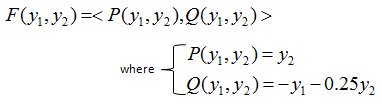
A system of two first order differential equations says how fast each variable changes at each state. That is exactly an arrow at each point of the (y₁, y₂) plane. So the equations define a vector field, and a solution is a curve that follows the arrows.

There is very important application of 'Vector Field'. You can get a solution to a differential equation without solving it if you use the vector field.

Let's see an example as shown below.

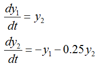
You can draw vector field from this set of differential equation by converting this equation into vector field format as shown below. As you see, just take the right hand side of differential equation and assign them to P(x,y) and Q(x,y) as shown below.

From the vector field plot for this equation, take any one point you want (This first point is the initial condition for the set of differential equation). Go to the end of the arrow (vector) and find another arrow which starts closest to it and then go to the end of the next arrow. If you repeat the process and draw a continous line you followed through, that becomes the solution of the different equation. (The red curve on the plot in the right hand is the path we can draw by this way). I put another note showing the step by step procedure of how this graph is drawn in slideshow and animation at my other note : www.freetechslide.com

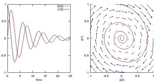
The two plots above show the same solution in two ways. On the left, y₁ and y₂ oscillate over time and slowly decay. On the right, the same solution is one red curve on top of the field. It starts at the initial condition, y₁ = 0 and y₂ = 1, at the top centre of the plot. From there it spirals clockwise toward the origin.

We can check the shape against the equations. The two equations together say y₁'' + 0.25 y₁' + y₁ = 0, which is a damped oscillator. Its characteristic roots are -0.125 +/- j0.992. So the amplitude decays as e^-0.125t, and one period takes about 2π/0.992 = 6.33 time units. At t = 25 the envelope is about e^-3.125 = 0.044, which matches the small oscillation at the right end of the left plot. The field also has divergence -0.25 everywhere, and a negative divergence means that areas in the plane shrink along the flow. That is why every path spirals inward.

Following is the matlab/octave code that produce the plots shown above. You can try with various other differential equations with this code. Just modify the parts in blue.

v = -1:0.2:1;
[y1,y2] = meshgrid(v);
u1=y2;
u2=-y1 - 0.25 .* y2;

dy_dt = @(t,y) [y(2);...
                        -y(1) - 0.25 .* y(2)];
odeopt = odeset ('RelTol', 0.00001, 'AbsTol', 0.00001,'InitialStep',0.5,'MaxStep',0.5);
[t,y] = ode45(dy_dt,[0 25], [0.0 1.0],odeopt);

subplot(1,2,1);plot(t,y(:,1),'r-',t,y(:,2),'b-'); xlabel('time'); legend('y2(t)','y1(t)');
subplot(1,2,2);
hold on;
quiver(y1,y2,u1,u2);
plot(y(:,1),y(:,2),'r-'); xlabel('y(2)');ylabel('y(1)');
axis([-1 1 -1 1]);
hold off;

Two labels in this listing do not match what it plots. The first is the legend. The command plot(t,y(:,1),'r-',t,y(:,2),'b-') draws y₁ in red and y₂ in blue, but legend('y2(t)','y1(t)') names them the other way around. The red curve starts at 0, which is y₁(0). So in the left plot, read the red curve as y₁ and the blue curve as y₂. The second is the axes of the right plot. The command plot(y(:,1),y(:,2),'r-') puts y₁ on the horizontal axis. But xlabel('y(2)') and ylabel('y(1)') label them the other way around. The shape of the curve is correct. Only the names are swapped.

• A system of first order equations is a vector field : the right hand sides are P and Q, and they give the direction of motion at every state.
• A solution is a path that follows the arrows : the initial condition picks the starting point, and the field decides the rest.
• Negative divergence means the paths spiral inward : for this example the divergence is -0.25, which is the damping term of the oscillator.