One of the most important assumption for most of communication theory is that the system is LTI (Linear Time Invarient). So it is very important to understand the concept of LTI before you start getting deeper into communication technology. In this page, I will explain about what 'Linear' (Linearity) means and why it is important and in another page I will explain about 'Time Invarience'.

• What does Linearity mean ?
• Why is a straight line not always linear ?
• What does a non-linear system look like ?
• Why is Linearity important ?
• Where does Linearity break in a real system ?
• Why does Linearity always appear with Time Invariance ?

What does Linearity mean ?

What does Linearity means ? you may think any function that can be expressed as a straight line in a coordinate system is linear. But it is not true. Not all straight line in the coordinate system is linear. For a function (system) to be a linear, it has to meet a criteria called 'principle of superposision'.

In short, the principle of superposition is to make the following equation true.

f(a+b) = f(a) + f(b)

Textbooks state a second condition beside that one, and it matters as much as the first. Scaling the input scales the output by the same factor, so f(k a) = k f(a) for any constant k. The two conditions are usually written on one line as f(k₁ a + k₂ b) = k₁ f(a) + k₂ f(b).

The two conditions together say a single thing. The system handles every input on its own, and it handles every input at the same strength. Nothing arriving at the input can change how the system treats anything else arriving with it.

This principle can be explained in an illustration as shown in Figure 1.

Let's assum that you have a function f(x) as a straight line starting starting from the origin (0,0) of the coordinate system.

Now look at the upper graph on left side first. If you plug a value 'a' (in thick blue line)' into the function. yoe will get the output of the function as f(a) (in thick red line).

Now look at the bottom graph on left side first. If you plug a value 'b' (in thick green line)' into the function. yoe will get the output of the function as f(b) (in thick black line).

Now let's take the graph of f(a+b). It is the graph on the right side. Just by looking, you would notice that f(a+b) is same as f(a) + f(b). Therefore, this graph(function, system) is linear.

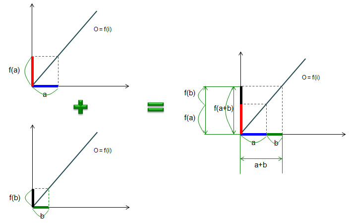
Figure 1. The two left hand panels are the same system driven twice, and the right hand panel is the system driven once with a+b. The stacked output brackets and the single f(a+b) bracket reach the same height, so superposition holds.

• Both axes belong to the system, not to the signal : the drawing labels the line O = f(i). The horizontal axis therefore carries the input, and the vertical axis carries the output. Every coloured segment on an axis is one level, not a waveform.
• The inputs are laid end to end : in the right hand panel the blue segment a and the green segment b sit on the input axis one after the other. The bracket underneath them measures a+b.
• The outputs stack the same way : the red f(a) sits below the black f(b) on the output axis. The f(a+b) bracket beside them reaches exactly the same height, and that equality is the whole picture.

As an example, let's take we have a function as follows.

f(x) = 2 x

Is this a linear function ? Let's see if this meets the principle of superposition, i.e, f(a+b) = f(a) + f(b). Let's assume a = 3, b = 2.

Then what is f(a) ? It is f(3) = 2 * 3 = 6

what is f(b) ? It is f(2) = 2 * 2 = 4

Then what is f(a+b) ? It is f(2+3) = f(5) = 5 * 2 = 10.

Is f(a+b) = f(a) + f(b) ? Yes, it is because f(3+2) = f(3) + f(2) = 6 + 4 = 10.

Does this satisfy the principle of superposition ? (In strict mathematics, you cannot prove it with just single. You have to prove this is true for any numbers... try all different values as 'a' and 'b' and check if it still works -:). But intuitively, you can say "Yes, it satisfy the principle of superposition, so this function is a linear'.

• Linear describes the system, not the shape on a graph : the test is whether superposition holds. A picture can suggest the answer, and only the test settles it.
• Two conditions, one idea : adding the inputs adds the outputs, and scaling the input scales the output. A system that fails either one is non-linear.
• One example never proves it : the warning above is the right one. Superposition has to hold for every pair of inputs, so a single pair of numbers can only disprove it.

Why is a straight line not always linear ?

The section above states that not every straight line is linear, and it does not say why. The reason is short, and the line it excludes is the one most readers try first. One example settles it.

Take f(x) = 2x + 1. It is a straight line, its slope never changes, and it looks like the safest function anyone could pick. Now run the same test the section above ran, with a = 1 and b = 2. Figure 2 sets that line beside f(x) = 2x and works the arithmetic through. The two lines have the same slope, and only one of them passes through the origin.

Figure 2. The offset is the whole difference. f(a) + f(b) evaluates the function twice and picks up the constant twice, while f(a + b) evaluates it once. A straight line is linear only when it passes through the origin.

• The origin is a test you can run by eye : a straight line through the origin is linear. A straight line that misses the origin is not, and nothing else in the picture decides the answer.
• The error equals the offset, not a fraction of it : f(a) + f(b) exceeds f(a + b) by c for every a and b. The mistake therefore stays the same size when the signal gets small.
• Scaling fails for the same reason : f(2a) is 5 here while 2 f(a) is 6, so the second condition breaks as well. One offset is enough to lose both.

Mathematicians have a name for this shape. A function of the form y = m x + c is called affine, and it is linear only when c is zero. Engineers rarely use the word, and they meet the case constantly.

The practical form of c is a DC offset. A constant voltage added somewhere in a receive chain is exactly this c, and it breaks superposition while bending nothing at all. It produces no harmonics and no compression, so the measurements aimed at non-linearity will not see it. Engineers therefore measure the offset and remove it first, and only then treat the rest of the chain as linear.

What does a non-linear system look like ?

If the explanation above is not clear to you, it would be clearer if you look at an example in which f(a+b) is not the same as f(a)+f(b). Following is an example.

Look at the function graph in this case. It is not the straight line, it is a path kinked at one point (or you can draw a curved line as the function).

Now look at the upper graph on left side first. If you plug a value 'a' (in thick blue line)' into the function. you will get the output of the function as f(a) (in thick red line).

Now look at the bottom graph on left side first. If you plug a value 'b' (in thick green line)' into the function. yoe will get the output of the function as f(b) (in thick black line).

Now let's take the graph of f(a+b). It is the graph on the right side. Just by looking, you would notice that f(a+b) is not same as f(a) + f(b). Therefore, this graph(function, system) is not linear.

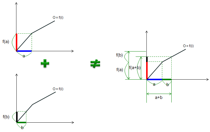
Figure 3. The same three panels as before, drawn on a function that bends at one point. The f(a + b) bracket on the right is visibly shorter than the stacked f(a) and f(b). The sign between the panels is the not-equal sign.

• The bend is the only change : the axes, the colours and the layout match the linear picture exactly. The line is steep below the bend and shallow above it, and that one difference produces everything else.
• The inputs still add, and the outputs no longer do : the blue a and the green b sit end to end on the input axis exactly as before. The input side of the test is unchanged.
• The shortfall has a visible cause : a + b lands beyond the bend, in the shallow region. Each unit of input buys less output there than it did below the bend.

As an example, let's take we have a function as follows.

f(x) = x^2

Is this a linear function ? Let's see if this meets the principle of superposition, i.e, f(a+b) = f(a) + f(b). Let's assume a = 3, b = 2.

Then what is f(a) ? It is f(3) = 3^2 = 9

what is f(b) ? It is f(2) = 2^2 = 4

Then what is f(a+b) ? It is f(2+3) = f(5) = 5^2 = 25.

Is f(a+b) = f(a) + f(b) ? No, it is because f(3+2) is 25 but f(3) + f(2) = 9 + 4 = 13.

Does this satisfy the principle of superposition ? No. So it is not a linear

The bend deserves a second look, because it is the shape a real device actually has. Below the bend each unit of input buys a fixed amount of output. Above it, the same unit buys less. A large input therefore lands in the shallow part and falls short of what the small signal behaviour predicted. An amplifier driven near its maximum output does exactly this, and a later section on this page returns to it.

• One counter-example is enough : f(x) = x² fails the test at a = 3 and b = 2, so the function is non-linear. Disproving superposition needs one pair of numbers, and proving it needs all of them.
• Squaring is the classic offender : it is the first term that breaks superposition in a polynomial model of a device. It is also the term that produces the second harmonic.
• The shortfall is not noise : the output falls below f(a) + f(b) every time rather than sometimes. The error is therefore a repeatable function of level, and averaging never removes it.

Why is Linearity important ?

I hope you have the general concept of linearity by now. But I think practically more important question would be "Why the Linearity is so important ?", "Why we have to care about linearity ?".

It is important because in linear system, once you have an output for any specific input, you can figure out all other outputs without doing real test.

For example, let's assume that you have a linear system and you know the outout of the system when you put '1' as an input is '2', i.e f(1) = 2 and somebody ask you to get the output when the input is 5, meaning that he wants to get 'f(5)'. In this case, by the principle of superposition you can rewrite the f(5) as follows.

f(5) = f(1) + f(1) + f(1) + f(1) + f(1)

Since you already know the value of f(1) = 2, you can get f(5) as follows without doing any test.

f(5) = f(1) + f(1) + f(1) + f(1) + f(1) = 2 + 2 + 2 + 2+ 2 = 10

You would see later that we usually indentify the characteristics of any linear system by what we call 'impulse response'. Once you have the impulse response of the system, you can figure out the output of the system for any input by using the impulse response. This is possible only when the system is Linear.

Let me say why that works, because the impulse response is the most reused idea in the whole subject. Any input can be written as a sum of impulses, with each one scaled and each one delayed. Linearity lets you add the responses to those impulses rather than measuring the combination. A sum of scaled and delayed copies of one response is convolution, and that is where the operation comes from.

The frequency domain reaches the same conclusion by another route. A linear system can change the amplitude and the phase of a frequency that reaches it. It can never produce a frequency that was absent from the input. That single restriction is why one curve of gain against frequency describes a filter completely. When a device emits harmonics, it has already told you that it is not linear.

Almost every technique on this site rests on the same assumption. Channel estimation measures the channel with a known signal and then applies the result to unknown data. That works only if the channel treats both the same way. An equalizer inverts the channel as a matrix or as a filter, and inverting anything requires the forward operation to be linear. Every MIMO precoder and every combining weight inherits the same requirement.

• One measurement covers every input : with superposition in place, the response to a single impulse predicts the response to everything else. Without it, every new input becomes a new experiment.
• A linear system moves energy and never creates a frequency : gain and phase can change, and the list of frequencies cannot. Harmonics at the output are direct evidence of non-linearity.
• The assumption is inherited rather than re-checked : channel estimation, equalization and MIMO all rely on it silently. When a receiver behaves oddly at high input level, test the assumption itself first.

Where does Linearity break in a real system ?

Every real device is non-linear somewhere, so the useful question is never whether a system is linear. The question is how far you can drive it before the answer changes. That distance is a design parameter, and it is paid for in power.

The transmit power amplifier meets the limit first, which is why the question has a cost at all. Figure 4 draws the transfer curve of a real amplifier against the straight line it is meant to follow. The two agree at low input, separate gradually, and end far apart.

Figure 4. The curve leaves the ideal line gradually rather than at a corner, so there is no single input level at which the amplifier stops being linear. The 1 dB compression point is the agreed marker, and back-off is the distance the designer keeps below it.

• The green band is where everything earlier on this page applies : inside it the red curve and the blue line almost coincide. Superposition holds closely enough there to use as a design assumption.
• The two curves separate smoothly : the transition has no corner. The amplifier gives a little less output than the line predicts, then a little less again, until it stops responding to more input at all.
• Back-off is a distance, and the operating point is a choice : the designer picks how far below the compression point the signal sits. That gap is the whole cost of linearity.

The damage from the bent region is worse than a little lost output. Put two tones into the amplifier and the curvature produces new tones at 2f₁ - f₂ and 2f₂ - f₁. These third order products sit immediately beside the original pair, so they land inside the channel or in the one next to it. A harmonic at 2f₁ is far away, so a filter removes it. No filter can remove a product that lands on top of the wanted signal. The amplifier page works this through with the polynomial model.

Two answers to this are in common use, and neither one is free. Back-off keeps the signal inside the straight part, so the amplifier delivers less output power for the same DC input and the efficiency falls. Predistortion shapes the input with the inverse of the measured curve, so the amplifier and the shaping together behave linearly over a wider range. Predistortion recovers some of the power that back-off sacrifices, and it costs processing and a calibration loop.

OFDM makes the problem harder rather than easier. An OFDM symbol is the sum of many subcarriers, and those subcarriers occasionally align in phase, so the waveform has short peaks far above its average. The average can sit deep inside the linear region while the peaks reach the compressed part. That gap is the reason peak to average power ratio is treated as a system parameter rather than a curiosity.

The receiver fails in the same way for a different reason. A strong interferer arrives with the wanted signal, drives the low noise amplifier or the analogue to digital converter past its range, and the converter clips. Clipping is the shape in Figure 3 with a hard corner instead of a gentle bend, and everything said there applies. This is why a receiver quotes a blocking specification and not only a sensitivity figure.

• Linearity is a range rather than a yes or a no : every amplifier is linear below some level and compressed above it. The number you need is that level, not the label.
• Intermodulation is worse than harmonics : a harmonic sits far from the wanted signal and a filter removes it. Third order products sit next to the wanted signal, and no filter separates them.
• Linearity and efficiency are bought from the same budget : back-off protects superposition by running the amplifier well below its maximum. That is exactly the power the designer wanted.
• The receive side has the same failure : a converter driven past full scale clips, and clipping breaks superposition as completely as compression does.

Why does Linearity always appear with Time Invariance ?

The two words are rarely used apart. Textbooks pair linearity with time invariance and then treat the pair as a single assumption called LTI, which is where this page opened. The two properties are independent of each other, and a system can satisfy one while failing the other.

Each property removes a different freedom from the system, and the table below sets them side by side.

Linearity removes the dependence on level, so the answer for one input predicts the answer for a scaled or summed input. Time invariance removes the dependence on the moment, so a measurement taken now is still correct later. One impulse response describes the system completely only when both hold. With linearity alone you would need a fresh impulse response for every instant. With time invariance alone you would need a fresh measurement for every input level.

Each half fails on its own in a case you already know. A radio channel with a moving terminal is linear and not time invariant. Adding two signals at the transmitter still adds them at the receiver, and the channel itself changes as the terminal moves. That is the reason reference signals are transmitted again and again rather than once per connection. A compressing amplifier is the opposite case, since it behaves identically at every moment and its gain still depends on the input level.

The other half of the pair has a page of its own, so Time Invariance covers the second property in the same detail. Read it next, and then read impulse response, which is the page where both assumptions are finally used.

• Two separate properties share one abbreviation : LTI joins them because the impulse response method needs both. Losing either one breaks the method, and it breaks it for a different reason each time.
• A fading channel is the everyday linear but time varying case : superposition holds at every instant, and the channel changes between instants. An estimate is therefore valid for a limited time rather than permanently.
• Check which half failed before fixing anything : when a fault depends on signal level, linearity is the problem. When it depends on the moment you measured, time invariance is. The two need different answers.