You may have seen so many different types of differential equations (e.g, linear homogenous, linear non-homogenous, non linear homogenous etc) and you might have seen a lot of different ways to solve the problem in symbolic (algebraic) method. But unfortunately there is no single method which can solve all of those types. Another issue with the algebraic method would be that it would be hard to use computer for the solutions. I think these two factors would have been strong motivations to rely on numerical solutions.
You would find many thick books which is only for solving differential equations in numerical methods, but we don't have to go through every page of those thick books. The underlining logic is pretty simple and with the solid understanding of the logic with some hands-on would help you go through those thick books much easily.
- How does a derivative become a step you can compute?
- How is the Duffing equation solved step by step?
- Why are numerical method books so thick?
How does a derivative become a step you can compute?
The first step of the numerical method came from what you learned from high school math (in my case) or from Pre-Calculus course. I assume that you know the following equation.
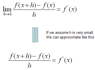
This defines on how we can convert the deferential form (f'(x)) into a simple rational form(non-differential form). This is the core of the numerical method. Once you got this form, you can easily convert almost any differential equations into the difference equations you can easily solve numerically.
Let's write this as a rule you can repeat. The lower equation in the diagram above is only approximately true, because h is small but not zero. So read its equals sign as "approximately equal". Multiply both sides by h and move f(x) to the right, and you get f(x + h) = f(x) + h f'(x). Now suppose the differential equation gives the derivative, y' = g(t, y). Then y(t + h) = y(t) + h g(t, y(t)). This one line is called the forward Euler method. Start from a known y(0), apply the line once, and you have y(h). Apply it again, and you have y(2h), and so on.
Every step makes a small error, because the curve bends between t and t + h. The error of one step is proportional to h2. You need 1/h steps to reach a fixed end time, so the total error is proportional to h. For example, take y' = -y with y(0) = 1. The exact value at t = 1 is e-1 = 0.36788. Euler with h = 0.1 gives 0.34868, an error of 0.0192. With h = 0.05 it gives 0.35849, an error of 0.0094. Halving h halves the error, as expected for a first order method.
Replace the derivative by a difference : f'(x) is approximately (f(x + h) - f(x))/h, and this turns a differential equation into an update rule.Forward Euler is one line : y(t + h) = y(t) + h g(t, y(t)), repeated from the initial value.The error shrinks with h : Forward Euler is a first order method. Its total error is proportional to h, so a ten times smaller h gives about a ten times smaller error.
How is the Duffing equation solved step by step?
Let's apply the rule to a real equation. The example is the Duffing equation, x'' + kx' + x3 = B cos(t). It describes a driven and damped oscillator with a cubic spring, and it has no closed-form solution. So the numerical method has to do all the work here.
For example, let's assume that we have a differential equation as follows (This is 2nd order, non-linear , non-homogeneous differential equation). I want to apply the converting equation shown above to this differential equation, but the converting equation we have is only for the first order differential form only. It was not for the second or higher order form.
Don't worry. By a few steps of mathematical manipulation, we can convert this 2nd order differential equations into a simultaneous differential equation which is made up of two first order differential equations. (In this way, you can convert any high order differential equations into a multiple first order differential equations. For example, you can convert 3rd order differential equation into three first order differential equations and you can convert 4th order differential equations into four first order differential equations).
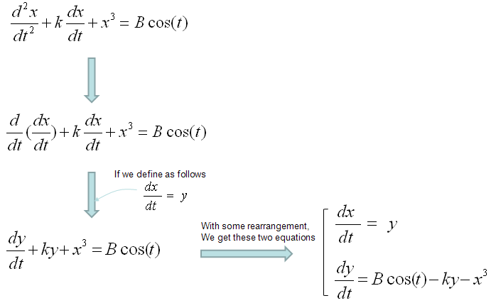
Once you get a set of first differential equations, you can easily get a set of equations as shown in step (3) by a simple mathematical manipulations. I would not verbally explain much about this process, just pick any of the differential equation and try this process on your own. Otherwise you would never understand this process. Use this example just as a cheatsheet when your memory fades away.
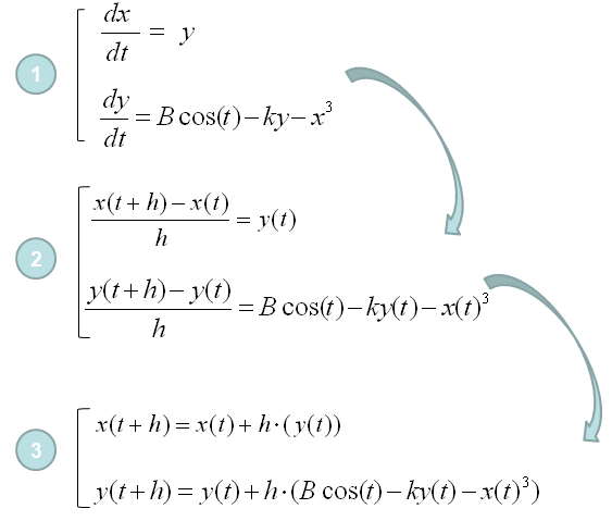
Once you get the set of multiple equations as shown in step (3), you can trace the values of each point of the solution by following procedure. I would not verbally explain much about this process, just pick any of the differential equation and try this process on your own. Otherwise you would never understand this process. Use this example just as a cheatsheet when your memory fades away.
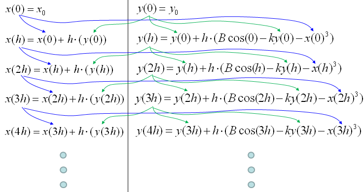
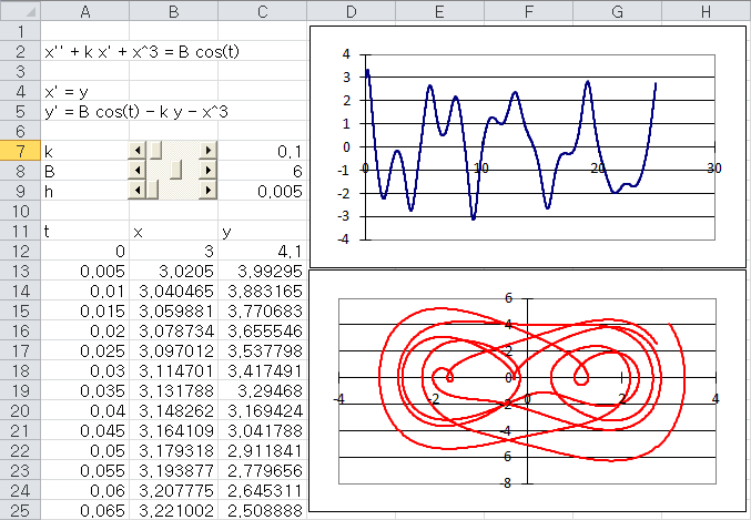
If you understood the logics shown just above, you can calculate each of the steps even with Microsoft Excel as shown below. I put the link so that you can download my spreadsheet but I strongly recommend you to try this on your own first.
Download this Excel File : Click here.
Let's check the first rows of the spreadsheet by hand. The settings are k = 0.1, B = 6, h = 0.005, x(0) = 3 and y(0) = 4.1. Step 3 gives x(h) = 3 + 0.005 * 4.1 = 3.0205. It also gives y(h) = 4.1 + 0.005 * (6 cos(0) - 0.1 * 4.1 - 33) = 4.1 + 0.005 * (-21.41) = 3.99295. Both values match the row for t = 0.005 in the sheet.
One small difference appears from the row for t = 0.01 onward. The sheet evaluates the forcing term at the new time, B cos(t + h), while step 3 in the diagram uses B cos(t). With cos(t), the y value in that row would be 3.883167 instead of 3.883165. Both versions are first order methods, and this difference is far smaller than the error of the method itself.
That error is not small for this equation. A comparison with an accurate solver shows it. Take scipy solve_ivp with a relative tolerance of 10-11 as the reference. With h = 0.005, the Euler value of x(t) differs from the reference by more than 0.1 already near t = 1, and by more than 0.5 near t = 14. Before t = 30 the difference reaches about 2.6, while x itself stays between about -3.1 and 3.3. So the later part of the plot in the sheet is not a close copy of the true solution. With h = 0.0005, ten times more steps, the largest difference over the same range drops to about 0.08.
One update line per first order equation : The Duffing equation becomes two first order equations, so each step updates x and y together.Each row uses only the previous row : This is why a spreadsheet is enough. Every cell formula refers to the row above it.Always test the step size : Run the calculation again with a smaller h. If the two results differ, the first h was too large.
Would this be simple enough for you ? If you say "No", it is true. If you say "YES", it would be true. It would take a little while and a certain amount of effort to understanding a new concept however simple it is. Just don't run away and give it a try.
Why are numerical method books so thick?
Somebody would ask "Is this all for getting numerical solutions for a differential equation ?". Is it realy simple like this to get a solution for any differential equations (ordinary differential equation, more specifically)? If it is the case, why our numerical method text book is so thick ?"
Good Question. Just in terms of concept of numerical method this is almost whole story, but in terms of applying this method to real life problems there are some practical issues with the basic method that I explained above.
i) Issue 1 : Sometimes there is a situation where the function (solution to the differential equation) can be very fast chaning function. For example, a function oscillating with high frequency. Of course you can still use the basic method explained above with very small 'h' value. But in this case, the amount of time you would need to get the solution will be very long. So it would be a little impractical in this case. If you are specifically interested in this issue and solution for it, try searching "Runge-Kutta" method.
ii) Issue 2 : Basically a numerical solution is to find a solution at many discrete points. It is not the continous solution. This gives you a problem. For example, let's assume that you got the solution of a differential equation at the points of independent variable (e.g x), x = 0.1, 0.2, 0.3, 0.4, 0.5 ..... What if I want to get the solution at x = 0.25 ? Do I have to calculate the whole process with h = 0.05 ? It is possible but it is impractical. Then how we get the solutions at the points that was not calculated ? The simplest and most widely used method is to use "interpolation" method.
In short, I would say your numerical method book for differential equation would get thick largely due to the two issues that I desribed above and I will explain these issues more detail (with illustrations) later. For now, understanding the basic process very clearly would be the highest priority.
Let's put names on the ideas behind those thick chapters, because these names are what you will search for. The first idea is a higher order method. Runge-Kutta methods evaluate the slope several times inside one step and combine the results. The classical fourth order method, RK4, has a total error proportional to h4. For y' = -y at t = 1, RK4 with h = 0.1 is off by only 0.00000033. Euler with the same h is off by 0.0192.
The second idea is an adaptive step. The solver estimates its own error at every step. It shrinks h where the solution changes fast, and it grows h where the solution is smooth. Matlab ode45 and scipy solve_ivp work this way, so you set a tolerance rather than a step size. This is the practical answer to Issue 1.
The third idea is stability. Some equations contain a very fast decaying part, and such equations are called stiff. Take y' = -50y. The exact solution decays, but forward Euler multiplies y by (1 - 50h) at every step. With h = 0.03 that factor is -0.5, and y decays. With h = 0.05 the factor is -1.5, and after 20 steps y has grown to about 3300. So stability limits the step size to h < 2/50 = 0.04, even where accuracy would allow a larger one. Implicit methods, such as backward Euler, remove this limit, and they are the usual choice for stiff problems.
The fourth idea is output between the steps. Modern solvers return a smooth interpolating polynomial with each step. This is the interpolation of Issue 2, built into the solver, and scipy calls it dense output.
Higher order methods : RK4 has an error proportional to h4, so it needs far fewer steps than Euler for the same accuracy.Adaptive step size : The solver picks h from an error tolerance, small where the solution changes fast and large elsewhere.Stiff equations : For explicit methods like forward Euler, stability rather than accuracy can set the largest usable h.Interpolation : Values between the computed points come from an interpolating polynomial, not from a new run with a smaller h.