Adjacency Matrix

Adjacency Matrix is a matrix which describes the connectivity among the nodes in a graph. (Google "Introduction to Graph Theory" or "Graph Theory Tutorial" if you are new to this area). The way you can construct the Adjacency Matrix from a graph is as follows. I hope this illustrations gives you the intuitive understanding without much description. Basic idea is to put "1" at the matrix element representing two points (from, to) if there is a connection for the two points and put "0" otherwise.

For a graph with n vertices, the adjacency matrix A is an n x n matrix. Row i and column i both belong to vertex i, so the element a_ij answers one question: is there an edge between vertex i and vertex j? I'll start with a directed graph, where the direction of the edge decides which of a_ij and a_ji gets the 1. Then the undirected case, the eigenvalue properties and the powers of A follow.

Adjacency Matrix for Directed Graph

Adjacency Matrix is a matrix that represents the connection among vertices. There can be two ways of representing the connection in matrix as in < Case 1 > and < Case 2 >. I think the typical way is < Case 1 > but < Case 2 > is also possible as long as you use the notation consistently in all the equations in which the matrix is used.

The two cases use the same graph, and the difference is only which index means the start of an edge. The graph has four vertices and four directed edges: 4 to 1, 1 to 3, 3 to 2 and 4 to 3.

Case 1

In Case 1, the columns are labeled From and the rows are labeled To. So an edge from vertex j to vertex i puts a 1 in row i, column j. The green lines in the drawing below connect each arrow to the element it produces.

Directed graph with four vertices and its adjacency matrix, columns From and rows To

Case 2

Case 2 swaps the roles, so the rows are From and the columns are To. The drawing below carries the same From and To labels and the same matrix as Case 1, so it does not show the swap. The table after the drawing gives the Case 2 matrix for this graph.

Directed graph with four vertices and its adjacency matrix, drawn with the same labels as Case 1

With the rows as From, the edge from vertex i to vertex j puts a 1 in row i, column j. The result is the transpose of the Case 1 matrix.

	To 1	To 2	To 3	To 4	row sum = out-degree
From 1	0	0	1	0	1
From 2	0	0	0	0	0
From 3	0	1	0	0	1
From 4	1	0	1	0	2

Most graph theory textbooks and the common software tools use the Case 2 form, with a_ij = 1 for an edge from i to j. The adjacency functions of MATLAB and of the Python package NetworkX both return this form. So check which form a text uses before you copy a formula from it. A formula written for one form needs A^T in place of A in the other form.

The row and column sums tell you the degrees. In the Case 2 form, the sum of row i is the out-degree of vertex i, and the sum of column j is the in-degree of vertex j. For this graph the out-degrees of vertex 1 to vertex 4 are 1, 0, 1 and 2, and the in-degrees are 1, 1, 2 and 0. In the Case 1 form, the two sums swap places.

A directed graph gives a matrix that is usually not symmetric : The edge 4 to 1 sets one element only, and the element for 1 to 4 stays 0.
Case 1 and Case 2 are transposes of each other : Either form works, as long as every equation on the page uses the same one.
Row sums and column sums give the out-degree and the in-degree : Which is which depends on the form, so read the labels first.

Adjacency Matrix for Non-Directed Graph

An undirected edge has no start and no end, so it sets two elements at once. The edge between vertex 1 and vertex 3 puts a 1 in a₁₃ and another 1 in a₃₁. The From and To labels therefore make no difference here.

The drawing below uses four vertices with four edges: 1-3, 1-4, 2-3 and 3-4. The blue arrows lead from each edge to the two elements it sets.

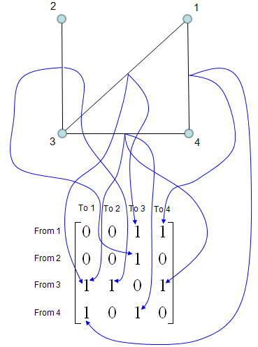
Undirected graph with edges 1-3, 1-4, 2-3, 3-4 and its symmetric adjacency matrix

Once you have the Adjacecy Matrix, you can do a lot of mathemtical operation for the matrix to find various useful information.

Three properties are visible directly in this matrix. First, the matrix is symmetric, so A = A^T. Second, the diagonal is all 0, because no edge starts and ends at the same vertex. A graph with a loop at vertex i puts a nonzero value in a_ii, and texts differ on whether that value is 1 or 2. Third, the sum of row i is the degree of vertex i. Here the degrees of vertex 1 to vertex 4 are 2, 1, 3 and 2. Their sum is 8, which is twice the number of edges, because every edge appears twice in the matrix.

An undirected graph gives a symmetric matrix : Each edge sets a_ij and a_ji together.
A zero diagonal means no loops : A simple graph has only 0 on the diagonal of A.
The sum of all elements is 2 x number of edges : For this graph that is 8 = 2 x 4. The row sums are the degrees, which the Degree Matrix puts on its diagonal.

Properties of Adjacency Matrix

Most properties of an adjacency matrix are statements about its eigenvalues. The eigenvalues do not depend on how the vertices are numbered, so they describe the graph itself rather than one particular matrix. The list below states the main ones, and the examples after it check them on the graphs of this page.

Even with the same graph, if lebeling (index) for each vertex is different, you may have different Adjacency Matrix. But the eigenvalues of all the adjacency matrix for the same graph is always same.
If the eigenvalues of two graphs do not match (are not same), then the graphs are not isomorphic. (But the converse is not true, meaning that there are cases where two graphs are not isomorphic but they have the same eigenvalues).
If the adjacency matrix is symetric, all of the eigenvalues of the matrix are real values.
If the adjacency matrix is symetric, it means that the graph is undirected.
If the adjacency matrix is symetric, all of the eigenvectors of the matrix is orthogonal to each other.

A renumbering of the vertices changes A into P^TAP, where P is a permutation matrix. This is a similarity transform, and that is why the eigenvalues stay the same. A classic pair shows that the converse fails. The star with one center and four leaves has the eigenvalues -2, 0, 0, 0 and 2. A 4-cycle plus one isolated vertex has exactly the same eigenvalues, but the two graphs are clearly not isomorphic.

The third bullet only works in one direction. The directed graph of Case 1 and Case 2 has no cycle, so a high enough power of its matrix is the zero matrix. Here A⁴ = 0, and all four eigenvalues are 0. They are real, but the matrix is not symmetric. For the undirected graph above, the eigenvalues are about -1.481, -1, 0.311 and 2.170, all real as the symmetric case requires. For the fourth bullet, keep in mind that a directed graph in which every edge has a reverse edge also gives a symmetric matrix. Such a graph is treated as an undirected graph. For the fifth bullet, when an eigenvalue repeats, its eigenvectors can be chosen to be orthogonal, but they do not have to be.

Eigenvalues belong to the graph, not to the numbering : Renumbering is P^TAP, which keeps the eigenvalues.
Equal eigenvalues do not prove isomorphism : The star with four leaves and the 4-cycle plus an isolated vertex share the eigenvalues -2, 0, 0, 0 and 2.
Symmetric means real eigenvalues, not the reverse : The directed example on this page has only zero eigenvalues and is not symmetric.

Application : Seeking connected path among vertice

The most common mathematical operation for the Adjacent Matrix is to take "Powers of the matrix". Following shows three matrix, A which is original adjacency Matrix and A^2 and A^3.

These three matrices belong to the undirected graph above, with the edges 1-3, 1-4, 2-3 and 3-4. Each one is symmetric, like A itself.

Adjacency matrix A of the undirected example with A squared and A cubed

Element value in A^2 is the number of possible paths connecting the two nodes represented by the element. If an element value is "1", it means there is only one path from one node to the other node that is represented by the element. If an element value is "2", it means there are two possible paths from one node to the other node that is represented by the element as illustrated below. In most case, only those elements with the value of "1" has practical meaning.

The drawing below marks two elements of A². The element in row 1, column 1 is 2, and the two boxes at the top show the two ways: 1-3-1 and 1-4-1. The element in row 1, column 2 is 1, and the box at the lower right shows the only way, 1-3-2.

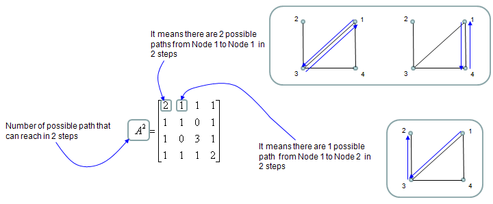
A squared with elements (1,1) = 2 and (1,2) = 1 explained by the 2-step routes on the graph

The rule behind this is that element (i, j) of A^k counts the walks of length k from vertex i to vertex j. A walk may visit a vertex more than once, so it is not always a path in the strict sense. Look at 1-3-1 above: it goes to vertex 3 and comes back. Element (1, 3) of A³ is 4, and all four walks repeat a vertex: 1-3-1-3, 1-3-2-3, 1-3-4-3 and 1-4-1-3. In this graph there is no route of length 3 from 1 to 3 that visits four different vertices. So every value in A^k has a meaning, not only the value 1.

Two more results come directly from the diagonal. The diagonal of A² is 2, 1, 3 and 2, which is the degree of each vertex, because each edge gives one walk out and straight back. The diagonal of A³ counts closed walks of length 3, and each of those goes around a triangle. The trace of A³ is 2 + 0 + 2 + 2 = 6. Each triangle is counted 6 times, 3 starting points in 2 directions, so this graph has 6 / 6 = 1 triangle. That triangle is 1-3-4.

A^k counts walks of length k : Element (i, j) is the number of k-step walks from vertex i to vertex j, including walks that revisit a vertex.
The diagonal of A² gives the degrees : For this graph it is 2, 1, 3 and 2, the same as the row sums of A.
trace of A³ / 6 counts triangles : Here 6 / 6 = 1, the triangle 1-3-4.
A zero element means no walk of that length : Element (2, 2) of A³ is 0, because vertex 2 lies on no triangle.

Examples on YouTube

The two videos below are useful if you prefer to see the construction worked on a board. The first one introduces graphs through walks and mail delivery routes. The second one comes from the MIT linear algebra course and treats the graph of a network as a matrix.