A rotation in 3D is easy to write down for one axis. A real object, however, usually turns around several axes at once. This page rotates a cube around the x, y and z axes in one step. It uses 4 x 4 homogeneous matrices, so the same machinery can add a translation later without any change. Let's build the combined matrix first, then read the result, and then look at the Matlab code that drew it.
- How is the three axis rotation matrix built ?
- What does the rotated cube look like ?
- Matlab Code
- Why does the order of the rotations matter ?
How is the three axis rotation matrix built ?
This is an example of rotating a 3D object (a Cube) using a Homogenous Matrix in the form as shown below. The transformation matrix is applied (multiplied) to each vertex of the cube. The three matrix (Rotating around each axis) is multiplied to all the vertices in sequence. The sequence of matrix multiplication is as shown below.
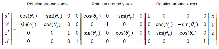
Figure 1. The three axis rotation in homogeneous form. The vertex on the right meets the x rotation first, then the y rotation, and the z rotation last.
- Each block rotates around one axis and leaves the coordinate of that axis unchanged. Rz keeps z, Ry keeps y and Rx keeps x. That is why each block has a lone 1 on the diagonal at the position of its own axis.
- The labels above the matrices follow the written order, z then y then x. The product is applied from right to left, so the order of application is x, then y, then z.
- The fourth row of every block is [0 0 0 1]. So the fourth coordinate d of the result stays 1, and the first three entries are the rotated x', y' and z'.
- The fourth column of every block is [0 0 0 1]T as well. A rotation has no translation part, so the origin, which is the centre of the cube, does not move.
- The y block has -sin(θy) in its first row and +sin(θy) in its third row. The right-hand-rule rotation around y has these signs the other way round. So this block is the right-hand rotation by -θy, and a positive θy turns the cube in the opposite sense to a positive θx or θz.
The example uses θx = π/3 (60 deg), θy = π/4 (45 deg) and θz = π/8 (22.5 deg). The Matlab code never shows the combined matrix, but it helps to see it once. Multiplying the three blocks gives the following matrix, rounded to four decimals.
Rz Ry Rx = [ 0.6533  -0.7571   0.0048   0 ]
           [ 0.2706   0.2276  -0.9354   0 ]
           [ 0.7071   0.6124   0.3536   0 ]
           [ 0        0        0        1 ]
Every vertex goes through this single matrix. For example, the corner (0.5, 0.5, 0.5) moves to (-0.0495, -0.2186, 0.8365). Its distance from the centre is 0.866 before and after the move, because a rotation never changes a length. You can also check this on the matrix itself. The upper-left 3 x 3 block R satisfies RRT = I and det(R) = 1, and these are the two conditions for a pure rotation.
Each axis has its own 4 x 4 block : the block keeps its own axis fixed and rotates the other two coordinates.The rightmost matrix acts first : in RzRyRxv, the x rotation reaches the vertex before the other two.The homogeneous coordinate stays 1 : the last row [0 0 0 1] guarantees it, so x', y' and z' can be read directly from the result.The y block on this page has the opposite sign convention : it is the transpose of the usual right-hand Ry, so a positive θy turns the other way.
What does the rotated cube look like ?
Numbers alone say little about a 3D rotation, so the example draws the cube before and after the transformation. Each state is drawn from four viewpoints. The three flat views are the easiest ones to check against the matrix, because each of them simply drops one coordinate.
The result of this example is as shown below.
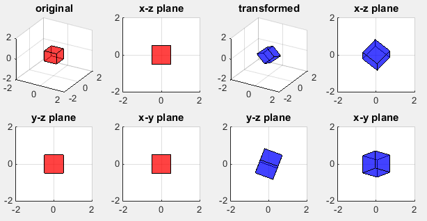
Figure 2. The cube before the rotation, in red, and after it, in blue. The rotated cube keeps its size and its centre, but none of its faces is parallel to a coordinate plane any more.
- The two left columns show the original cube. The 3D view uses view(30,30), and the flat views look along the y axis (x-z plane), the x axis (y-z plane) and the z axis (x-y plane). The cube is aligned with the axes, so it appears as the same 1 x 1 square in all three.
- The two right columns show the rotated cube in the same four views. Its faces are tilted, so each flat view shows the outline of several faces at once.
- The outline grows, but the cube does not. In the x-z view the rotated cube reaches about +/-0.71 in x and +/-0.84 in z, compared with +/-0.5 before.
- The centre stays at the origin in every view, because the matrix has no translation column.
You can predict these outline sizes from the matrix without plotting anything. For a unit cube centred at the origin, the half width along x is half the sum of the absolute values in the first row of R. That gives 0.5 x (0.6533 + 0.7571 + 0.0048) = 0.708. The same rule with the third row gives 0.5 x (0.7071 + 0.6124 + 0.3536) = 0.837 for z, and the second row gives 0.717 for y. These are the extents that Figure 2 shows.
A rotation keeps the shape and the centre : only the orientation changes, so a larger outline in a flat view is a projection effect.Flat views are the fastest check : each view drops one coordinate, so it can be compared with two rows of the matrix.The outline width follows from the matrix rows : half the sum of the absolute values in a row is the half width of the rotated unit cube along that axis.
Matlab Code
Following is the MatLab code for this example. For now, don't pay too much about the code itself, just focus on number marked in red and try to undertand the mathematical meaning intuitively. You can just copy the code here into your Matlab and change the numbers in red part until you develop the intuitive understanding.
Note : When copy and paste this code, '...' may cause some error. In that case, erase '...' and retry '...' in your matlab editor.
clear all;

vert = [-0.5 -0.5 -0.5;  ...
        -0.5 0.5 -0.5;  ...
         0.5 0.5 -0.5;  ...
         0.5 -0.5 -0.5; ...
        -0.5 -0.5 0.5; ...
         -0.5 0.5 0.5;  ...
          0.5 0.5 0.5; ...
          0.5 -0.5 0.5];

fac = [1 2 3 4; ...
    2 6 7 3; ...
    4 3 7 8; ...
    1 5 8 4; ...
    1 2 6 5; ...
    5 6 7 8];

% original object
subplot(2,4,1);
patch('Faces',fac,'Vertices',vert,'FaceColor','r');
axis([-2 2 -2 2 -2 2]);
grid();
material shiny;
alpha('color');
alphamap('rampdown');
view(30,30);
title('original');

% view along y-axis (x-z plane)
subplot(2,4,2);
patch('Faces',fac,'Vertices',vert,'FaceColor','r');
axis([-2 2 -2 2 -2 2]);
grid();
material shiny;
alpha('color');
alphamap('rampdown');
view(0,0);
title('x-z plane');

% view along x-axis (y-z plane)
subplot(2,4,5);
patch('Faces',fac,'Vertices',vert,'FaceColor','r');
axis([-2 2 -2 2 -2 2]);
grid();
material shiny;
alpha('color');
alphamap('rampdown');
view(90,0);
title('y-z plane');

% view along z-axis (x-y plane)
subplot(2,4,6);
patch('Faces',fac,'Vertices',vert,'FaceColor','r');
axis([-2 2 -2 2 -2 2]);
grid();
material shiny;
alpha('color');
alphamap('rampdown');
view(0,90);
title('x-y plane');

% transforming object
VerticesHom = zeros(8,4);
for i = 1:8
    VerticesHom(i,:) = [vert(i,:) 1];
end

phiX = pi/3;
TxMatrixX = [1    0       0        0;...
            0 cos(phiX) -sin(phiX) 0; ...
            0 sin(phiX) cos(phiX)  0; ...
            0     0       0        1];

phiY = pi/4;
TxMatrixY = [cos(phiY)  0 -sin(phiY) 0;...
             0          1      0     0; ...
             sin(phiY)  0  cos(phiY) 0; ...
             0          0       0    1];

phiZ = pi/8;
TxMatrixZ = [cos(phiZ) -sin(phiZ)  0  0;...
             sin(phiZ) cos(phiZ)   0  0; ...
             0         0           1  0; ...
             0         0           0  1];

TxVerticesHom = TxMatrixZ * TxMatrixY * TxMatrixX * VerticesHom';
TxVerticesHom = TxVerticesHom';

TxVertices = zeros(8,3);
for i = 1:8
    TxVertices(i,:) = TxVerticesHom(i,1:3);
end

% transformed object
subplot(2,4,3);
patch('Faces',fac,'Vertices',TxVertices,'FaceColor','b');
axis([-2 2 -2 2 -2 2]);
grid();
material shiny;
alpha('color');
alphamap('rampdown');
view(30,30);
title('transformed');

% view along y-axis (x-z plane)
subplot(2,4,4);
patch('Faces',fac,'Vertices',TxVertices,'FaceColor','b');
axis([-2 2 -2 2 -2 2]);
grid();
material shiny;
alpha('color');
alphamap('rampdown');
view(0,0);
title('x-z plane');

% view along x-axis (y-z plane)
subplot(2,4,7);
patch('Faces',fac,'Vertices',TxVertices,'FaceColor','b');
axis([-2 2 -2 2 -2 2]);
grid();
material shiny;
alpha('color');
alphamap('rampdown');
view(90,0);
title('y-z plane');

% view along z-axis (x-y plane)
subplot(2,4,8);
patch('Faces',fac,'Vertices',TxVertices,'FaceColor','b');
axis([-2 2 -2 2 -2 2]);
grid();
material shiny;
alpha('color');
alphamap('rampdown');
view(0,90);
title('x-y plane');
The listing does four things in order. First, vert holds the eight corners of the cube, one corner per row, and fac lists the four corners of each of the six faces. Second, the loop appends a 1 to each corner. This turns vert into the 8 x 4 matrix VerticesHom of homogeneous coordinates. Third, the red lines build the three blocks of Figure 1 and apply them in one statement. Fourth, the result is cut back to three columns and drawn with patch.
The transposes around the red statement are easy to miss. VerticesHom stores one vertex per row, but the matrices in Figure 1 act on column vectors. So the code multiplies by VerticesHom', which holds one vertex per column, and then transposes the result back. Without them Matlab reports a dimension error, because a 4 x 4 matrix cannot multiply an 8 x 4 matrix.
The red numbers are the three angles. A good first experiment is phiX = 0 and phiY = 0, so that only the z rotation acts. The x-y view then shows the square turned by 22.5 deg, while the other two views show rectangles about 1.31 wide and 1 high.
The data layout and the math layout differ : the data holds one vertex per row, the matrices expect one vertex per column, and the transposes convert between the two.The appended 1 makes the 4 x 4 product possible : the code drops it again before plotting.Change one angle at a time : a single nonzero angle gives a rotation that you can predict and check in the flat views.
Why does the order of the rotations matter ?
The page multiplies the blocks in the order RzRyRx. So a natural question is whether another order would give the same cube. It does not, because matrix multiplication is not commutative, and 3D rotations are the best-known example of that.
Let's compare the two orders with the same three angles. The reversed product RxRyRz gives a different matrix.
Rx Ry Rz = [ 0.6533  -0.2706  -0.7071   0 ]
           [-0.3744   0.6963  -0.6124   0 ]
           [ 0.6581   0.6648   0.3536   0 ]
           [ 0        0        0        1 ]
Only the top-left and the bottom-right elements of the 3 x 3 part agree. The corner (0.5, 0.5, 0.5) now lands at (-0.1622, -0.1453, 0.8382) instead of (-0.0495, -0.2186, 0.8365). The difference is small here, but it grows with the angles. Take 90 deg around x and 90 deg around y, with the blocks of Figure 1. The top face normal (0, 0, 1) ends up along -y when x is applied first, and along -x when y is applied first.
The product also has two readings. RzRyRxv rotates around the fixed x axis first, then the fixed y axis, then the fixed z axis. Read from left to right, the same product rotates around z first and then around the already rotated y and x axes of the body. Both readings give the same final cube, so you only need to state which one you use.
One more fact makes the chain easier to understand. Any product of rotations is itself one rotation around a single axis. For the matrix of this page, cos(angle) = (trace(R) - 1)/2 = 0.117, so the angle is 83.3 deg. The axis is the eigenvector of R for the eigenvalue 1, which points along (-0.779, 0.354, -0.517) up to sign. So the three turns of the example could be replaced by one 83.3 deg turn around that axis.
Rotation matrices do not commute : RzRyRx and RxRyRz give different results for the same angles.Three angles alone do not define an orientation : the order of the axes, and whether they are fixed or body axes, must be stated too.Any chain of rotations is one rotation : its axis is the eigenvector for the eigenvalue 1, and its angle follows from the trace.