I have several example that I like for Matrix. Some of the examples, I like them in terms of Modeling which means 'converting a real life problem into a matrix format' and some of the examples, I like them in terms of visualization of the matrix. This example is the one I like in terms of modeling.
The model on this page is called a Markov chain, and its matrix is called a stochastic matrix, or a transition matrix. Each entry is a fraction that moves from one entity to another in one round. Let's build the matrix from a diagram, run it for many rounds, and then see why the result settles to fixed values.
- How is the interaction written as a matrix ?
- What happens after many rounds of interaction ?
- Why does the result stop changing ?
- Examples on YouTube
How is the interaction written as a matrix ?
Let's say you have three different entities and all of these three entities interact each other. Every time they interact each other, it gives some portion of what it has to another states and it gets some portioin from other entities. One example with a specific number is as follows. For example, if you look at the entity (2) and entity(1). You would see that these two entities gives something to each other and takes something from each other. More specifically, for every round of interaction, entity (2) gives 40 % of what it has to entity (1) meaning that entity (1) takes 40 % from engity (2) and entity (1) gives 80 % of what is has to entity (2), meaning entity (2) takes 80% from entity (1).
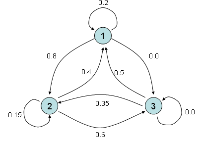
Figure 1. Three entities and the fractions that flow between them in one round. A loop on a node is the fraction that the entity keeps.
If you describe the relationship between each entity verbally as I described above, you would notice that very soon it gets very complicated and you would forget what you described about entity (1),(2) when you describe entity (2),(1). Furthermore, in most of real life problems the number of entities being involved in the problem tend to be much more than 3. In this case, it is almost impossible to describe all the possible relationships in verbal form. But if you use the matrix form, you can describe this kind of situation in a very simple manner as follows.
Each row number represents the entities where an arrow (shown above) starts and each column represents the entities where an arrow ends. The number within the matrix represents how much amount of things transfers from an entities to another entities. For example, if you see the point where row (2) and colum (3) meets, you see the number '0.6'. It means that for every round of interaction, entity (2) transfer 60 % of what it got to entity (3).
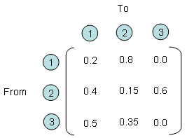
Figure 2. The same diagram as a transition matrix. Row i lists what entity i sends, and column j lists what entity j receives.
- Row 1 is [0.2 0.8 0.0]. Entity 1 keeps 20 %, sends 80 % to entity 2 and sends nothing to entity 3. These are the loop on node 1 and its two outgoing arrows in Figure 1.
- Row 2 is [0.4 0.15 0.6]. Entity 2 sends 40 % to entity 1 and 60 % to entity 3, and the loop on node 2 is labelled 0.15.
- Row 3 is [0.5 0.35 0.0]. Entity 3 sends 50 % to entity 1 and 35 % to entity 2, and the loop on node 3 is labelled 0.0.
- The diagonal holds the loops, which are the fractions each entity keeps. The off-diagonal entries are the arrows.
A transition matrix has one rule that is easy to check. Each entity can only give away what it has, so every row must add up to exactly 1. Row 1 does, with 0.2 + 0.8 + 0.0 = 1. Row 2, however, adds up to 1.15, and row 3 adds up to 0.85. So entity 2 gives away more than it has, and entity 3 loses 15 % without sending it anywhere.
The two loop labels in Figure 1 appear to be swapped. Entity 2 already sends 40 % + 60 % = 100 % to the other two entities, so it cannot keep 15 % as well. If entity 2 keeps 0.0 and entity 3 keeps 0.15, every row adds up to 1. The rest of this page uses the matrix as drawn and also this corrected matrix, so that you can see what the row rule does.
as drawn                        corrected loops

[ 0.2   0.8   0.0  ]  sum 1.00    [ 0.2   0.8   0.0  ]  sum 1
[ 0.4   0.15  0.6  ]  sum 1.15    [ 0.4   0.0   0.6  ]  sum 1
[ 0.5   0.35  0.0  ]  sum 0.85    [ 0.5   0.35  0.15 ]  sum 1
Rows are senders and columns are receivers : the entry in row i and column j is the fraction that moves from entity i to entity j in one round.Every row of a stochastic matrix adds up to 1 : an entity keeps or sends exactly what it has, nothing more and nothing less.Check the row sums before using the matrix : here they show that the loop labels of entities 2 and 3 are swapped in the diagram.
What happens after many rounds of interaction ?
OK.. Now I have a matrix representing how each of entities in a system interact each other. So what ? How can I use this matrix ?
I said this matrix represents the interactions among each entities for each round of interaction. What if this kind of interaction repeats 100 times ? If entity (1) had 100, entity (2) has 500 and entity (3) has 300, how much they would get after 100 times of interaction ?
Can I get the answers to all of these questions from this matrix ?
In conclusion, the answer is YES. and then How ? It is simple, just multiply the same matrix 100 times (Matrix multiplication, not a scalar multiplication) and then you would get the answer for this. Again, you don't have to multiply the matrix 100 times by your hand. Just leave it to the computer.
Again, converting a real life problem into a Matrix format is your job and doing mathemtical operation for solution finding is not your job. It's computer's job.
One detail is missing from "multiply the same matrix 100 times". The amounts that the entities hold also enter the calculation. Write them as the row vector x0 = [100 500 300]. One round is the product x1 = x0P, where P is the transition matrix. The vector stands on the left, because the rows of P are the senders. After k rounds the amounts are xk = x0Pk, so 100 rounds need the matrix power P100.
Let's run the first round with the corrected matrix. Entity 1 receives 100 x 0.2 + 500 x 0.4 + 300 x 0.5 = 370. Entity 2 receives 100 x 0.8 + 500 x 0.0 + 300 x 0.35 = 185, and entity 3 receives 500 x 0.6 + 300 x 0.15 = 345. The total is still 900. The table below follows the amounts further.
round k    entity 1   entity 2   entity 3   total
   0        100.0      500.0      300.0      900
   1        370.0      185.0      345.0      900
   2        320.5      416.8      162.8      900
   5        317.9      340.2      241.9      900
  10        320.0      340.0      240.0      900
 100        320        340        240        900
The amounts swing strongly in the first rounds and then settle at 320, 340 and 240. After about ten rounds they change only in the second decimal place, and they stay there. So the answer to the 100-round question is 320, 340 and 240, and it would be the same after 1000 rounds.
The matrix as drawn behaves differently. After one round the amounts are 370, 260 and 300, and the total has grown from 900 to 930. The total then keeps changing, and after 100 rounds it is about 11,200, with no fixed values in sight. The reason is the row sum 1.15 of entity 2, which creates new material every round. A model like this is not a Markov chain, and its long-run answer has no physical meaning.
The state is a row vector on the left of P : xk+1 = xkP, so k rounds give x0Pk.A correct stochastic matrix keeps the total : the amounts move between the entities, but they always add up to 900.The amounts settle to fixed values : with the corrected matrix they reach 320, 340 and 240 after about ten rounds.A wrong row sum changes the total : the matrix as drawn grows the total from 900 to about 11,200 in 100 rounds.
Why does the result stop changing ?
The table above raises a question. Why do the amounts stop at 320, 340 and 240, and why do they stop at all? The answer is an eigenvector of the transition matrix, and it also gives a way to find the final values without running 100 rounds.
The amounts stop changing when one more round gives the same vector, that is, when πP = π. So π is a left eigenvector of P for the eigenvalue 1, or, in the more usual form, an ordinary eigenvector of PT. A stochastic matrix always has the eigenvalue 1, because every row adds up to 1. For the corrected matrix, the three equations of πP = π have the solution π = (16, 17, 12)/45 = (0.356, 0.378, 0.267). This is the fraction of the total that each entity holds in the end. Multiplied by 900, it gives exactly 320, 340 and 240.
The other two eigenvalues decide how fast the amounts settle. For the corrected matrix they are -0.325 +/- j0.211, and both have the magnitude 0.387. In each round, the part of xk that differs from the steady state shrinks by roughly this factor. After 10 rounds that is 0.38710, which is about 10-4, and after 100 rounds nothing of it is left. That is also why every row of P100 equals (0.356, 0.378, 0.267). The final values therefore do not depend on the starting amounts, only on their total.
This does not happen for every stochastic matrix. It is guaranteed when some power of P has only positive entries, and such a matrix is called regular. The corrected matrix qualifies, because P2 already has no zero entry. A counter example is the 2 x 2 matrix [0 1; 1 0], which swaps the two amounts in every round and never settles.
The steady state is an eigenvector : πP = π makes π the eigenvector of PT for the eigenvalue 1.The final share of each entity is fixed : here it is (16, 17, 12)/45, which gives 320, 340 and 240 out of 900.The second largest eigenvalue sets the speed : a magnitude of 0.387 makes the deviation about 10-4 of its size after 10 rounds.Convergence needs a regular matrix : some power of P must have only positive entries, or the amounts can keep oscillating.
Examples on YouTube
The two videos below explain Markov chains and Markov matrices with more examples.
Other Links