Even though a same signal is transmitted from single transmission antenna, the signal may go through various different path. Each of the different path may cause different travel distance if the signal get reflected by one or more obstacles (like buildings) and in some case different path may has different physical property of propagation media, so it is higly likely that the signal traveling through different path would arrive at the reciever antenna at different timing. So if you send a signal from a transmitter antenna and measure the arrival time at the reciever antenna which is a certain distance away from the transmitter antenna, you would get multiple different arrival timing.

• Representation in Channel Impulse Response
• Max Delay Spread
• Problems with Max Delay Spread
• Average Delay Spread
• Variance of Delay
• RMS Delay Spread
• Working the numbers on one example channel
• From RMS delay spread to coherence bandwidth
• What the number is actually used for
• Typical values, and where they come from
• Reference :

If you plot those arrival timing on the axis of time, you would see a certain variation (spread) of those values. This spread is called 'Delay Spread'.

In other words,  delay spread refers to the time difference between when the first and last copies of a signal arrive at the receiver when multipath propagation occurs. Multipath propagation is when the signal takes different paths from the transmitter to the receiver, resulting in multiple copies of the signal arriving at different times. The delay spread measures how spread out in time these different signal copies are. A large delay spread means the multiple copies arrive over a longer time period, while a small delay spread means the copies arrive within a shorter time span. So the delay spread gives an indication of the dispersion or spreading of the signal over time caused by taking different paths from transmitter to receiver. The larger the delay spread, the more dispersed the signal is when it arrives.

I think this is enough for the definition for layman. If you want to dig into further details and go through some mathematical model of these delay spread see the following.

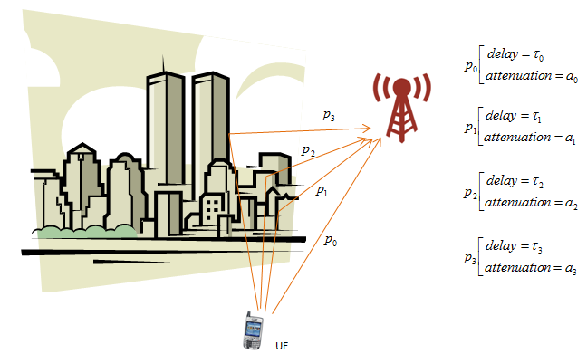
• The UE sits at the bottom of the drawing and the base station antenna sits at the right. Four orange arrows leave the UE and reach the antenna, labelled p₀ to p₃.
• The paths are not the same length. Path p₀ runs almost straight, while the others bend around the buildings of the skyline and therefore travel further.
• Each path is described on the right by two numbers in a bracket, a delay and an attenuation. Path i carries delay = tau_i and attenuation = a_i.

Those two numbers per path are the whole channel, as far as this page is concerned. Everything that follows is a way of reducing the set of them to a single figure that describes the channel.

Note which way round the drawing is. The UE transmits and the base station receives, so this is the uplink, and the same picture holds in the other direction. The Channel Model page works through what the transmitted signal becomes once these paths are added up.

Representation in Channel Impulse Response

The channel impulse response(CIR) shows the output of a communications channel when the input is an impulse or spike. It basically captures the effect of the channel on the signal. In wireless communication, where signals take multiple paths from transmitter to receiver, the CIR provides information about these different multipath components.

The CIR plot has spikes that represent the different paths the signal takes. The timing or position of each spike on the x-axis shows the delay for that path. The height of the spike on the y-axis indicates the amplitude or strength of that path.

• The x-axis typically represents time (or delay).
• The y-axis represents amplitude.

So the overall CIR pattern with its spikes spaced out in time shows the response of the wireless channel to an input impulse. The spikes characterize the various multipath components - their timing (delay) and strength (amplitude). This helps understand how the wireless channel impacts the signal based on the different paths taken.

CIR plot the signals detected by a reciever antenna in time vs amplitude plot. it can be represented as follows. As you see here, you will see multiple copies of the same signal coming in with different timing and different amplitue. Using these time variation and amplitude variation, we can defined several different criteria (metrics) to define the nature of the channel. To introduce these criteria (metric) is the main purpose of this page.

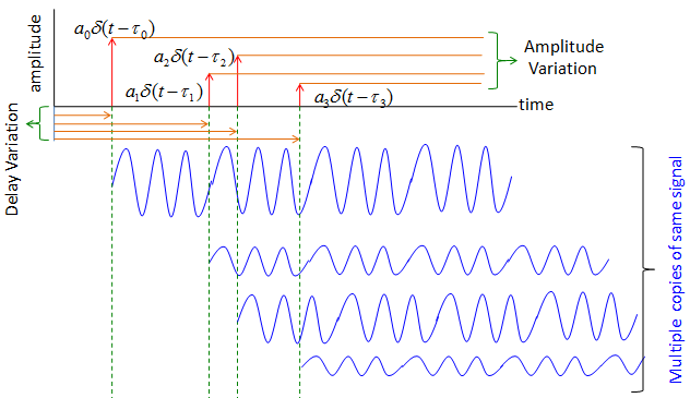
• The upper plot is the impulse response. Four red impulses stand on the time axis, written a₀δ(t-tau₀) through a₃δ(t-tau₃), one per path.
• The green brace at the upper right is labelled Amplitude Variation, and it gathers the heights of the four impulses. The green brace at the left is labelled Delay Variation, and it gathers their positions along the time axis.
• The lower half of the drawing shows what those impulses mean for a real waveform. Four copies of the same blue burst are stacked, each starting later than the one above it and each weaker.
• The green and black dashed verticals tie the two halves together. Every dashed line runs from one impulse down to the start of the copy that impulse describes.

The bracket on the right names the point of the lower half : multiple copies of the same signal. The transmitter sends nothing new for each copy, and the receiver still has to separate them.

Two independent variations are therefore on display, and the rest of this page keeps them apart. The delay variation sets how far the arrivals are spread in time, and the amplitude variation sets how much each arrival matters. A metric that uses only the first of them is the next section.

Max Delay Spread

The simplest thing to measure on an impulse response is the distance between its two ends. It ignores the weighting and it ignores the power, so the answer follows from the first arrival and the last one alone. That measurement has a name.

The maximum delay spread is a way to quantify the time dispersion or spreading effect of the wireless channel based on the CIR.

To find it from the CIR plot:

• Look for the earliest notable peak or spike in the CIR - this represents when the first significant multipath component arrives.
• Then look for the last major peak - this will be the last multipath component to arrive.
• The time delay between the first and last major spikes is the maximum delay spread.

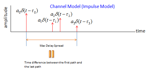
• The plot is titled Channel Model (Impulse Model) and carries the same four impulses as the drawing above, from a₀δ(t-tau₀) at the left to a₃δ(t-tau₃) at the right.
• The orange double arrow below the axis runs from the first impulse to the last one and is labelled Max Delay Spread.
• The note under the arrow states the definition in words : the time difference between the first path and the last path.

Read the arrow carefully, because it touches only two of the four impulses. The two in the middle could move anywhere between the ends, or disappear altogether, and the arrow would not change length.

Max Delay Spread measures the full time extent over which the multipath arrivals are spread out, from the earliest to the latest component. The wider this spread, the more dispersion in time the channel causes.

The maximum delay spread is useful because it characterizes the full dispersive effect of the channel. Knowing the extent of the delays can help design systems and set requirements to handle the time distortion caused by the wireless channel.

Problems with Max Delay Spread

Max Delay Spread is a very simple in terms of definition and measurement. But it would not be a good metric (indicator) represeing the property of a channel.

Issues of Max Delay Spread as a channel property metric is illustrated below.

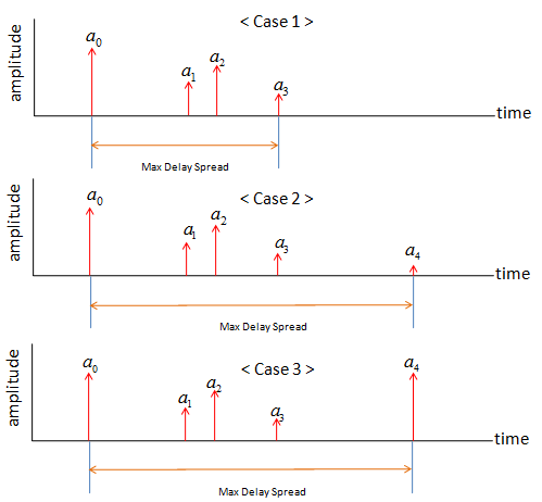
Case 1: This seems to show a typical channel impulse response where the multipath components (arrows) are relatively close together in terms of delay (time axis). The amplitude of these components might vary, but they're clustered within a specific time range.

Case 2: Here, most of the multipath components are clustered similarly to Case 1, but there's an outlier(a4)—a late-arriving component. This outlier significantly extends the max delay spread, even if its amplitude might be low.

Case 3: The multipath components in this case also seem to span a delay range similar to Case 2. However, the amplitudes of these components, especially the late-arriving ones(a4), seem to be different from those in Case 2.

The difference between the two lower panels is worth stating as it is drawn, because it is easy to miss at a glance. In Case 2 the arrow for a₄ is short, so the late path is weak. In Case 3 the arrow for a₄ reaches almost the height of a₀, so the late path carries as much power as the first one.

Max delay spread reports the same number for both panels. A metric that weighted each arrival by its power would separate them, and that is exactly what the next section introduces.

From these cases, we would notice some issues of using Max delay spread as follows. (NOTE : These would not be issues only for Max Delay Spread. It can be an issue of any types of delay spread, but the issues is more profound in Max Delay Spread comparing to other types like average delay spread or RMS Delay spread etc)

Impact of Outliers:

Case 1 provides a more "conventional" view of a channel, where the max delay spread might be a reasonably accurate representation of the channel's time dispersion.

Case 2 highlights the limitation of using max delay spread as a sole metric. A single outlier can distort the perceived channel property significantly.

>Amplitude Variations:

Even though Cases 2 and 3 might have a similar max delay spread, their channel characteristics could be quite different due to amplitude variations. This difference can impact system performance in terms of ISI, signal strength, and the effectiveness of mitigation techniques.

Average Delay Spread

To overcome the limitation of the Max Delay Spread (i.e, the distortion by outlier, no consideration of power), a new terms was introduced. It is 'Average Delay Spread' or 'Mean Delay Spread' Just jumping to conclusion, the term 'Average Delay Spread' in reality reprsented by 'Weighted Average Delay Spread' and the term 'Weighted' indicates 'Power Weighted'.

NOTE : Why the 'Power' term is introduced in this definition ?

The inclusion of this term is important for several reasons:

• Prioritizes Significant Paths: Weighting by power means paths with stronger signals contribute more to the average. This appropriately emphasizes components that have a larger impact on the received signal.
• Models Real-World Behavior: Power weighting reflects that early arrivals often have higher strength while late arrivals are attenuated. This matches real-world channel characteristics.
• Physical Meaning: The power-weighted average delay indicates the center of gravity for multipath arrival times, based on the distribution of signal energies.
• Relevance for Performance: Power-weighted metrics like RMS delay spread correlate better with channel effects on system performance like intersymbol interference.
• Consistency: Using power matches other channel models and metrics that account for path amplitudes, like the channel impulse response.

Now lets look further into the details of mathematical representation of Average Delay Spread (This note is mainly based on the videos listed under Reference section)

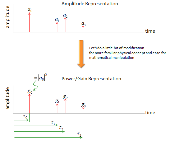
First let's revise a little bit of channel impulse response plot as shown below. There is no changes on time delay part, but definition of amplitude part is changed a little bit. I reprsented the amplitude in the unit of power.

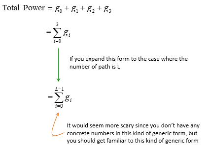
Based on the defintion shown above, total power can be represented as below. This is simple.. just sum of the power of all multipath component. We need this 'Total Power' at the normalization step that comes later.

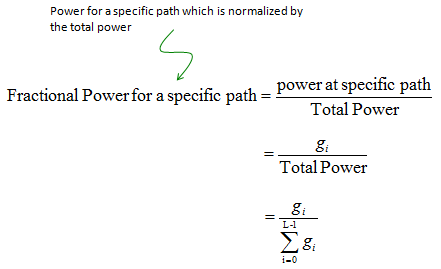
We can normalize the power of each multipath component with the Total Power as shown below. This normalized power is called as Fractional Power.

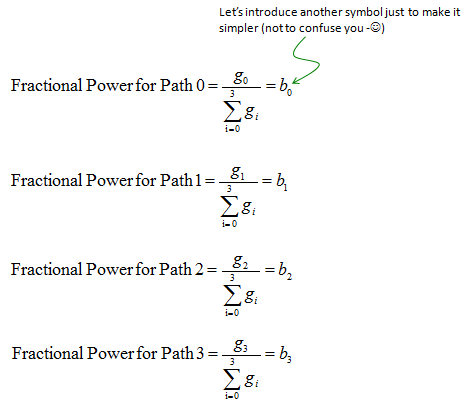
Applying this to the specific example channel response plot shown above, we can represent the Fractional Power for each component as follows

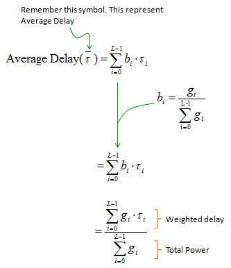
Now we can define using the fractional power term and delay term as shown below.

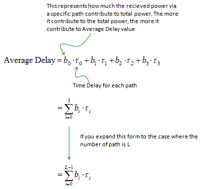
Definition itself is good enough with the equation shown above. But if you want to include fractional power in original form (blown out form), you can rewrite the equation as shown below.

Variance of Delay

The "Variance of Delay" in a communication system, especially in a multipath environment, quantifies the spread or dispersion of individual path delays around the mean or average delay. It provides an insight into the variability or inconsistency in the delays experienced by signals or packets as they traverse different paths.

The variance of delay quantifies the spread or dispersion of these different delays. A large variance implies a wide spread of delays, while a small variance means the delays are clustered close together.

So in simple terms, variance of delay characterizes how much the different multipath delays deviate from the average delay. It directly impacts the dispersion of the received signal in time domain. A large variance causes more smearing of the signal, while a small variance preserves the signal shape.

Knowing the variance of delay helps determine the type of equalization needed to combat multipath effects in communication systems. It is an important parameter for modeling multipath channels.

NOTE :  how variance of delay helps determine the type of equalization ?

Equalization techniques are used to combat this dispersion and reconstruct the original signal. The type of equalizer needed depends on the amount of expected delay spread, which is characterized by the variance of delay.

Specifically:

• If the variance of delay is small (delay spread is insignificant), then a simple equalizer like a linear transversal equalizer is sufficient. The taps can cover the small expected delay spread.
• If the variance of delay is moderate, an adaptive equalizer like decision feedback equalizer (DFE) works better. The feedback loop can track moderate variations in delay spread.
• If the variance is large (delay spread is very long), more advanced techniques like maximum likelihood sequence estimation (MLSE) are required. The equalizer must consider multiple symbol intervals to cover the long delay spread.
• So in summary, estimating the variance of delay from channel measurements gives an indication of the severity of multipath dispersion. This helps select the optimal equalizer structure and complexity to undo the channel distortions. A larger variance requires more complex equalizers to handle the extensive delay spread.

Knowing the variance of delay therefore guides the system designer towards choosing the right equalization strategy for the given multipath conditions.

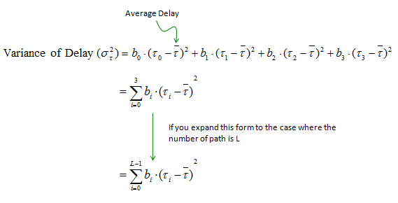
Mathematical representation of Variance of Delay is as follows. The b0,...,b3 is the weighting factor that are derived in the same way as explained in Average Delay.

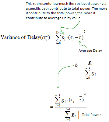
If you want to include fractional power in original form (blown out form), you can rewrite the equation as shown below.

RMS Delay Spread

RMS delay spread is a metric used to characterize the multipath propagation delay in a wireless channel. It quantifies the amount of delay dispersion experienced by a signal as it propagates through different paths from transmitter to receiver.

Mathematically, RMS delay spread is defined as the square root of the second central moment(i.e, variance or spread around the mean) of the power delay profile.

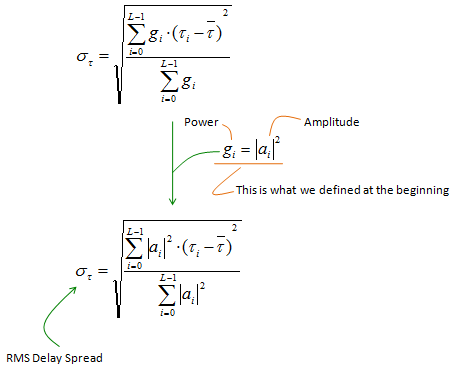
• The upper equation gives sigma_tau as a square root. Under the root sits the sum of g_i(tau_i - tau_avg)² divided by the sum of g_i, which is the variance of the section above. The figure draws tau_avg as tau with a bar over it.
• The middle note substitutes g_i = |a_i|², and marks it as what was defined at the beginning. Power on the left, amplitude on the right.
• The lower equation is the same expression after that substitution, so it is written in the amplitudes a_i that a measurement produces directly.

The two forms are one equation, and which one to use depends only on what the measurement hands over. A power delay profile gives g_i and suits the upper form. A channel estimate gives complex taps and suits the lower one.

In simple terms, RMS delay spread is the standard deviation of the different multipath delays, weighted by the power in each path.

A larger RMS delay spread implies the multipath delays are more spread out, causing greater symbol smearing and inter-symbol interference. Smaller values indicate clustered channel taps.

The RMS Delay Spread provides an indication of the multipath richness of the environment and the coherence bandwidth of the channel. A larger RMS Delay Spread indicates a more dispersive channel with a lower coherence bandwidth, which can affect the performance of wireless communication systems.

Working the numbers on one example channel

The three definitions above are easier to trust once they have produced an actual number. The table below takes one four path channel and carries it through every step of the sections above, from the powers to a single figure for the spread.

The delays and the powers are invented, and the unit of power does not matter. Every power is divided by the total in the next column, so the fractional power b_i comes out the same whether the entries are milliwatts or watts.

Three numbers come from the last two columns. The average delay is the total of the fifth column, 0.380 μs. The variance is the total of the sixth, 0.2476 μs², and its square root is the RMS delay spread, 0.498 μs.

The max delay spread needs neither column. It is the last delay minus the first, so it is 1.6 μs.

Compare those two figures before going further. Max delay spread reports 1.6 μs and RMS delay spread reports 0.50 μs, which is more than a factor of three apart. Both describe the same channel, and neither is wrong. They answer different questions.

The last column also answers a question the Problems section raised. Path 3 carries a tenth of the total power and contributes 60 percent of the variance, because the squared distance from the average delay grows faster than the weight shrinks. Path 0 contributes 29 percent and path 2 contributes 11 percent.

Path 1 contributes almost nothing, and the reason is worth noticing. Its delay of 0.4 μs sits within 0.02 μs of the average delay, so its squared distance is near zero whatever its power. A path near the centre of gravity moves the variance hardly at all.

The warning the page gives about outliers therefore survives the move to RMS. Power weighting stops one weak late path from dominating the way it does in max delay spread, and it does not remove the effect. The page says as much in its own note above, and this table puts a figure on it.

From RMS delay spread to coherence bandwidth

The section on RMS delay spread closes by naming coherence bandwidth without saying how the two connect. The connection is a reciprocal, and it is the main reason the RMS figure is measured at all.

Delay spread is a time domain measurement. Its frequency domain counterpart asks a different question : over how wide a band does the channel stay roughly constant. That width is the coherence bandwidth, written B_c.

A long echo means the paths interfere differently at different frequencies, so the response varies quickly across the band. A short echo means the opposite. B_c is therefore roughly 1 / sigma_tau, and the channel of the table above gives about 2 MHz.

The constant in front of that reciprocal depends on how much correlation is demanded. A common convention puts B_c at about 1 / (5 sigma_tau) for 0.5 correlation and about 1 / (50 sigma_tau) for 0.9. Those two turn the 2 MHz above into 400 kHz and 40 kHz. Quote the assumption alongside the number, or the number means little.

What the figure decides is whether a channel counts as flat or frequency selective. A signal narrower than B_c meets one gain across its whole band and fades as a unit. A signal wider than B_c meets a different gain at each end, and no single correction fixes both.

Run a 20 MHz carrier through the example channel and the answer is immediate. The coherence bandwidth is 2 MHz at the most generous convention, so the carrier is ten times too wide, and the channel is frequency selective. That is the ordinary case in cellular radio rather than the exception.

The Coherence page takes the same reciprocal from the other direction, alongside coherent time, and the Channel Model page works through what a frequency selective channel does to the received symbols.

What the number is actually used for

A channel metric is worth measuring only when it changes a design decision. Delay spread changes three of them, and the first is the one most visible in a specification table.

An OFDM system prefixes every symbol with a copy of its own tail, called the cyclic prefix. Echoes arriving within that prefix overlap the copy rather than the symbol before it, so the receiver can discard the prefix and lose nothing. Echoes arriving after it leak into the previous symbol and cannot be undone.

The prefix length is therefore chosen against the delay spread of the channels the system is meant to work in. This is the one decision where the max figure is the right one rather than the RMS figure, because a prefix that covers the average still lets the tail through.

LTE fixes two lengths. The normal cyclic prefix runs about 4.7 μs and the extended one about 16.7 μs. A cell with echoes beyond 4.7 μs is therefore a reason to configure the longer prefix and pay the overhead it costs. NR keeps the same idea and scales the prefix with the subcarrier spacing, so 15 kHz gives roughly the LTE figure and each doubling of the spacing halves it.

That scaling is less alarming than it looks. A high subcarrier spacing is used at high carrier frequencies and in small cells, where the delay spread is short for the reasons the next section gives. The extended prefix survives at one numerology only, and the Numerology page carries the table that says which.

The second decision belongs to single carrier receivers, and the Variance of Delay section above already states it. A small spread needs a linear equalizer, a moderate one needs a decision feedback equalizer, and a large one needs sequence estimation. The metric picks the structure before any hardware is built.

The third decision is pilot spacing. A channel estimate measured on one subcarrier stays usable across about one coherence bandwidth, so the reciprocal of the section above sets how far apart pilot subcarriers can sit. A longer echo means closer pilots, and closer pilots mean less room for data.

Typical values, and where they come from

The sections above define delay spread without saying what it measures out at in practice. The answer moves by three orders of magnitude between ordinary environments. One constant fixes the scale, and everything else follows from geometry.

Radio travels 300 m in 1 μs. A delay spread of 1 μs therefore means the longest useful path runs about 300 m further than the shortest. A spread of 30 ns means a difference of about 10 m. Every figure below is that arithmetic applied to a room, a street or a valley.

Indoors the reflectors are walls and furniture, so the extra path lengths are metres and the spread lands in the tens of nanoseconds. An office or a home typically measures somewhere between 20 and 100 ns, which is why a wireless LAN can use a short guard interval.

An outdoor urban cell reflects off buildings a few hundred metres apart, so the spread rises to hundreds of nanoseconds and into the low microseconds. Hilly and mountainous terrain is worse again, because a reflector kilometres away still returns enough energy to matter, and several microseconds are possible.

Carrier frequency moves the answer in the opposite direction. At millimetre wave the reflections lose far more energy at each bounce, and the beams are narrow. Fewer paths survive, so the spread is shorter than at low band in the same place. The short cyclic prefixes of the high numerologies rest on exactly this.

Simulation work does not pick these numbers by hand. 3GPP TR 38.901 models delay spread as a random variable, and its distribution depends on the scenario. The tapped delay line and clustered delay line profiles are then scaled by a chosen delay spread value. The named scaling steps run from very short to very long, and a study picks the one its scenario calls for.

The Propagation Modeling page covers those models and where the parameters come from. Treat the ranges here as orders of magnitude rather than as specification values, because a measured channel in any one location can sit well outside the usual band for its category.

Reference :

[1] Lecture 20: Max Delay Spread

Prof. Aditya K. Jagannatham

Dept. of Electrical Engineering

[2] Lecture 21: RMS Delay Spread

Prof. Aditya K. Jagannatham

Dept. of Electrical Engineering

[3] Lecture 22: Delay Spread and Inter Symbol Interference

Prof. Aditya K. Jagannatham

Dept. of Electrical Engineering