The Duffing oscillator is a well-known and widely studied system in nonlinear dynamics, often used to illustrate complex behaviors such as bifurcations and chaos. It serves as a quintessential example of how simple nonlinear systems can produce rich and sometimes unpredictable dynamics. Typically, it models a damped oscillator with a nonlinear restoring force and an external periodic driving force. Although the specific notation and parameter names can vary slightly across different texts and studies, the underlying structure of the equation remains fundamentally the same. The system's sensitivity to initial conditions and parameter values makes it a powerful demonstration tool for exploring the transition from regular motion to chaotic regimes in physics and engineering.

Build Up Intuition

Before diving into theory, I would like you to have a chance to play with this simple simulation and build your own intuition about the dynamics of the Duffing oscillator. Building up intuition is important because it grounds abstract mathematical concepts in visual and experiential understanding. Especially in nonlinear systems like this, where small parameter changes can lead to dramatically different outcomes, intuition helps you recognize patterns, anticipate behaviors, and grasp the qualitative nature of stability, bifurcation, and chaos—long before equations reveal them formally. By interacting with the system directly, you train your mind to connect cause and effect in dynamic environments, which is essential not just for learning, but for creativity and problem-solving in complex systems.

Following is usage of this program.

Starting the Visualization

• Open DuffingOscillator.html in a modern web browser
• Click the "Start" button to begin the simulation
• Click "Pause" to temporarily stop the simulation
• Use "Reset" to return to initial conditions

Parameter Controls

• α (Alpha): Controls the linear stiffness term
• β (Beta): Controls the nonlinear stiffness term
• δ (Delta): Controls the damping coefficient
• γ (Gamma): Controls the amplitude of periodic forcing
• ω (Omega): Controls the frequency of periodic forcing
• Initial Conditions: Set x₀ and ẋ₀ for different starting points

Visualization Options

• Time Series Plot: Shows x and ẋ vs time
• State Space Plot: Displays the phase portrait (x vs ẋ)
• Trail Length: Adjust how many points are shown in the plots (100 to 100,000)
• Color Scheme: Choose from:
  • Rainbow
  • Fire
  • Ocean
  • Grayscale

Preset Configurations

• Default: Standard parameter set
• Chaotic Attractor: Shows chaotic behavior
• Period Doubling: Demonstrates period-doubling bifurcation
• Soft Spring: Models a softening spring system
• Hard Spring: Models a hardening spring system
• Escape from Well: Shows escape from potential well
• Period-3 Orbit: Displays a period-3 solution

Zoom Controls

Both Time Series and State Space plots have independent zoom options:

• Both Axes: Zoom affects both x and y axes
• X-Axis Only: Horizontal zoom only
• Y-Axis Only: Vertical zoom only

Additional Features

• Mouse coordinates are displayed in the bottom-right corner
• Save the current view as an image using the "Save Image" button
• Adjust the time step for simulation accuracy (0.001 to 0.05)
• Real-time parameter adjustment
• Smooth animation with configurable trail length

There is another way of visuallizing the chaotic behavior of a system. Poincare map is the one. A Poincaré map offers a powerful way to visualize the complex behavior of dynamical systems, especially in the context of chaos. Unlike traditional time series plots that show how a variable evolves over time, or state space trajectories that illustrate continuous paths through a system's phase space, a Poincaré map samples the system at discrete intervals—typically once per forcing period in a driven oscillator. This results in a scatterplot that condenses high-dimensional behavior into a two-dimensional slice, making it easier to identify periodicity, bifurcations, or chaotic regimes. While time series and state space plots help us see the continuous evolution of motion, the Poincaré map captures the underlying structure of that motion, offering a more distilled view of long-term dynamics and stability.

Followings are the description on how you play with this program

Parameters

The Duffing oscillator is defined by the equation:

ẍ + δẋ + αx + βx³ = γcos(ωt)

Adjustable parameters:

• α (alpha): Stiffness coefficient [-2 to 2]
• β (beta): Nonlinear stiffness [0 to 10]
• δ (delta): Damping coefficient [0 to 1]
• γ (gamma): Forcing amplitude [0 to 10]
• ω (omega): Forcing frequency [0.1 to 2]
• x₀: Initial position
• ẋ₀: Initial velocity

Simulation Controls

• Preset Settings: Choose from predefined configurations:
  • Default Chaotic
  • Period Doubling
  • Double Periodic
  • Single Scroll
• Integration Parameters:
  • Steps/Period: Number of integration steps per forcing period
  • Total Periods: Total number of periods to simulate
  • Transient: Number of initial periods to discard
• Display Options:
  • WebGL: Toggle WebGL acceleration
  • Grid: Toggle grid display

Interactive Features

• Mouse Control:
  • Zoom: Mouse wheel
  • Pan: Click and drag
  • Coordinates: Real-time position display
• Simulation Control:
  • Start/Pause: Control simulation
  • Reset: Return to initial conditions
  • Save: Export current view as image

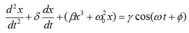
How it works ?

The Duffing oscillator is a well-known example of a system used to demonstrate chaotic behavior and dynamics. It is represented mathematically by a second-order differential equation that incorporates terms for displacement, velocity, and nonlinear restoring forces. The general form of the equation is:

The meaning of each terms and coefficients are as follows :

x = displacement

dx/dt = velocity

d²x/dt² = acceleration

δ = damping coefficient

ω0 = natural frequency of oscillation

β = nonlinearity coefficient

γ = forcing amplitude

ω = forcing frequency

φ = phase shift of forcing function

Here, each term and coefficient has a specific meaning. The variable x represents displacement, dx/dt represents velocity, and d²x/dt² represents acceleration. The parameter δ is the damping coefficient, which quantifies the system's resistance to motion. The terms β and ω₀ describe the nonlinear and natural frequency of oscillation, respectively. The forcing term γ cos(ωt + φ) accounts for an external periodic force, where γ is the forcing amplitude, ω is the forcing frequency, and φ is the phase shift of the forcing function.

The characteristics of the Duffing oscillator arise from the nonlinearity introduced by the x³ term. This nonlinearity enables the system to exhibit chaotic behavior under certain conditions. Depending on the parameter ranges, the oscillator may display bounded, periodic oscillations or chaotic dynamics. Varying the forcing frequency ω relative to the natural frequency ω₀ has a significant impact on the behavior of the system. As parameters are adjusted, the oscillations may switch between regular periodic motion and chaotic trajectories.

An important feature of the Duffing oscillator is its sensitivity to initial conditions. Even slight changes in the starting values can result in vastly different trajectories over time. The phase shift φ of the external forcing function plays a crucial role in determining when chaotic regimes emerge.

To explore the behavior of the Duffing oscillator, tools like phase portraits and Poincaré sections can be used. These visualizations reveal the underlying attractors of the system and help illustrate its transition between order and chaos. By numerically solving the equation and experimenting with different parameters and initial conditions, one can observe how the system evolves and how its dynamics change in response to external influences.

The characteristics of this equation can be summarized as follows :

• The x3 term introduces nonlinearity which enables chaotic dynamics.
• The system exhibits chaotic, bounded oscillations for certain parameter ranges.
• Varying the forcing frequency ω relative to the natural frequency ω0 impacts the behavior.
• The oscillations switch between periodic and chaotic as parameters change.
• Slight changes in initial conditions yield dramatically different trajectories over time.
• The phase shift φ of the external forcing alters when chaotic regimes emerge.
• Tools like phase portraits and Poincar sections reveal the underlying attractor.

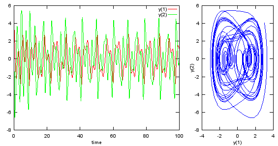
You can plot out the solution of this equation using a simple script below. Play with parameters and initial conditions and see how the plot changes.