The Lorenz attractor is one of the most iconic visualizations in chaos theory, illustrating how deterministic systems - those governed by precise laws - can nonetheless exhibit unpredictable and seemingly random behavior. It was first discovered by Edward Lorenz, a meteorologist, in 1963 while studying simplified equations to model atmospheric convection. He developed a system of three coupled, non-linear differential equations to describe the motion of fluid under certain thermal conditions. These equations track how three variables - commonly denoted as x(t) (convection rate), y(t) (horizontal temperature variation), and z(t) (vertical temperature variation) - evolve over time.

Despite their simplicity, the Lorenz equations exhibit sensitive dependence on initial conditions, a hallmark of chaotic systems. This means that even a minute change in starting values can lead to drastically different outcomes over time. This sensitivity is often metaphorically captured by the phrase "the butterfly effect," suggesting that the flap of a butterfly’s wings in Brazil could set off a tornado in Texas.

Graphically, the Lorenz attractor forms a strange attractor - a fractal structure in 3D space that resembles the shape of butterfly wings. Rather than converging to a fixed point or a periodic orbit, the trajectories of the system spiral indefinitely around two focal points, never repeating and never escaping. This shows how deterministic rules can lead to long-term unpredictability, blurring the line between order and chaos.

The Lorenz attractor has since become a foundational model not just in meteorology, but in a wide range of disciplines—from fluid dynamics and engineering to biology, neuroscience, and even economics - where complex, dynamic systems are studied. It reminds us that complexity does not always require complexity in laws, but can emerge from the recursive interaction of simple rules.

• Build up Intuition
• How it works ?
• What happens when rho changes ?
• How fast do two nearby paths separate ?

Build up Intuition

Before diving into the mathematical intricacies of the Lorenz system, it's helpful to first develop an intuitive understanding of how the system behaves and what role each parameter plays. One effective way to do this is by interacting with a simple simulation program that visualizes the system's evolution over time. By observing how the system responds to changes in parameters, you can gain a hands-on feel for the dynamics at play. This approach makes it easier to grasp the deeper concepts behind the equations, and it bridges the gap between abstract mathematics and real-world behavior. Instead of jumping straight into theory, let’s first explore how simple tweaks in the parameters influence the overall pattern and motion - this will build a strong foundation for understanding the fascinating chaotic behavior that follows.

The system is described by three coupled differential equations:

dx/dt = σ(y - x)

dy/dt = x(ρ - z) - y

dz/dt = xy - βz

Where:

• σ (sigma) is the Prandtl number, representing the ratio of kinematic viscosity to thermal diffusivity
• ρ (rho) is the Rayleigh number, related to the temperature difference between the top and bottom of the system
• β (beta) is a geometric factor related to the size of the system

This is the usage of this program.

Parameters Control

The three parameters are the coefficients of the equations above. A change takes effect on the next step, and the path continues from its current point with the new values. So you can watch one path change its behavior. For example, lower Rho to 20, and after a while the path settles onto one fixed point.

• Sigma (σ): Controls the rate of convection (default: 10)
• Rho (ρ): Controls the temperature difference (default: 28)
• Beta (β): Controls the ratio of box dimensions (default: 2.67)

Initial Conditions

These three values set the start point (X0, Y0, Z0) of the path. The program reads them only when the simulation restarts, so press Reset after you change them. A small change gives a different path but the same butterfly shape, and the last section of this page measures how fast two such paths separate.

• X0: Initial X coordinate (default: 0.1)
• Y0: Initial Y coordinate (default: 0)
• Z0: Initial Z coordinate (default: 0)

Visualization Options

The time step is the size of one RK4 integration step, and the program takes one step per animation frame. So a larger step makes the path grow faster on screen. It also changes the computed path itself. Runs with 0.01 and 0.005 from the same start agree until about t = 24 and then separate. The WebGL option currently only restarts the simulation, because the 3D view always uses the WebGL renderer of three.js.

• Color Scheme: Choose between Rainbow, Fire, Ocean, and Grayscale
• Time Step: Adjust simulation speed (0.001 to 0.05)
• WebGL Toggle: Enable/disable WebGL rendering

Camera Controls

The camera controls move your view of the 3D path, and they never change the numbers. The program also draws the x-y, x-z and y-z projections in separate panels. So you can compare a rotated 3D view with the flat views, and with the Matlab plots further down this page.

• Left Mouse: Rotate view
• Right Mouse: Pan view
• Mouse Wheel: Zoom in/out
• Reset View: Return camera to default position

Actions

The three buttons control the run as a whole. The program starts on its own when the page loads, so the first press of Start/Pause pauses it. Reset clears the path and starts again from X0, Y0 and Z0, and it is the step that applies new initial conditions.

• Start/Pause: Toggle simulation
• Reset: Clear and restart simulation
• Save Image: Capture current view as image

How it works ?

Lorenz attractor is obtained by solving a system of non-linear differential equation numerically as shown below. If you plot the solution of each single variable (fuction) on time domain (i.e, x(t), y(t), z(t)) you would see a pretty much radom like plots, but if you plot any of the two variables (or 3 variables) in parametric plot, you would see some pattern as shown below. The exact trajectory for each function(variable) changes very unpredictable way as you change the initial value by even very small degree, you would still see very similar overall plot. This is why the solution of the system equation is called as an attractor.

The image below writes the same three equations with other letters. P stands for σ, r for ρ and b for β, and each right side is multiplied out. For example, σ(y - x) becomes -Px + Py. The two terms xz and xy are the only nonlinear parts of the system.

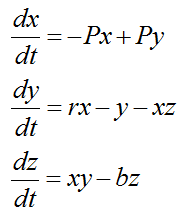
Figure 1. The Lorenz equations with P, r and b. The products xz and xy are the only nonlinear terms, and chaos needs them.

Here, P, r, and b are parameters that define the behavior of the system, such as the Prandtl number, Rayleigh number, and a geometric factor. The parameters shown in this equation maps to the parameters shown in the program in previous section as follows

• P = sigma
• r = Rho
• b = Beta

Physical Interpretation of the Parameters

Understanding the physical interpretation of the parameters in the Lorenz system is essential for grasping how this seemingly simple model gives rise to chaotic behavior. Each parameter—sigma (σ), rho (ρ), and beta (β)—has a concrete meaning rooted in fluid dynamics and thermodynamics. These constants are not arbitrary; they represent specific physical properties of the system such as the ratio of momentum to thermal diffusion, the strength of buoyancy-driven convection, and geometric characteristics of the environment. By examining how these parameters influence the evolution of the system’s variables, we gain deeper insight into the mechanisms that drive instability, feedback loops, and ultimately, the emergence of chaos.

σ (Sigma) – Prandtl Number

Definition:

σ = ν / α

where:

ν is the kinematic viscosity (momentum diffusivity)

α is the thermal diffusivity (heat diffusivity)

Physical Meaning:

• Sigma (σ) measures the relative effectiveness of momentum diffusion compared to heat diffusion.
• It reflects how quickly velocity changes (due to viscosity) spread out compared to temperature changes.

Interpretation:

• Low σ → thermal diffusion dominates (heat spreads faster than momentum)
• High σ → momentum diffuses more efficiently than heat
• A common value used in simulations is σ = 10.

Effect on the Lorenz System:

σ controls the coupling between the x and y variables, influencing how rapidly the fluid responds to thermal gradients with motion.

ρ (Rho) – Rayleigh Number

Definition:

ρ = Ra / Ra_c, where Ra = (g β_T ΔT d³) / (ν α)

where:

• g is gravitational acceleration
• β_T is the thermal expansion coefficient
• ΔT is the temperature difference between the top and bottom
• d is the depth of the fluid layer
• ν is kinematic viscosity
• α is thermal diffusivity
• Ra_c = π⁴(1 + a²)³ / a² is the critical Rayleigh number, where a is the aspect ratio from the β definition below. For a² = 1/2 it is about 657.5, and convection starts at ρ = 1.

Physical Meaning:

• Rho (ρ) quantifies the intensity of thermal forcing relative to damping effects.
• It measures how strongly buoyancy drives convection in the system.

Interpretation:

• Low ρ → no convection
• Critical ρ → convection starts
• High ρ → turbulence or chaos develops

Effect on the Lorenz System:

ρ determines the transition from stable to chaotic behavior, controlling the strength of instability in the system.

β (Beta) – Geometric Factor

Definition:

β = 4 / (1 + a²)

where a is a system-specific geometric ratio (e.g., aspect ratio of convection cells)

Physical Meaning:

Beta (β) reflects the vertical structure of the system, specifically how vertical temperature gradients influence motion.

Interpretation:

• Large β → stronger damping of vertical fluctuations
• Small β → slower decay, more vertical variability

Effect on the Lorenz System:

β influences how quickly the z variable (vertical temperature deviation) evolves and stabilizes.

Numerical Solution of the Equation

When solved numerically, the solutions to these equations - x(t), y(t), and z(t) - appear random when plotted individually over time. However, when plotted in a parametric space (e.g., plotting x versus y, y versus z, or x versus z), the solutions reveal a fascinating and intricate pattern. This pattern, known as the Lorenz attractor, has a characteristic butterfly shape and is deterministic yet highly sensitive to initial conditions.

This sensitivity means that even a minuscule change in the initial values of x, y, or z leads to vastly different trajectories over time, a hallmark of chaotic systems. Despite this unpredictability in the exact trajectories, the overall structure of the attractor remains consistent. This robustness is why the Lorenz attractor is called an "attractor": it "attracts" the system's state into a specific, complex pattern that persists over time, regardless of small perturbations in the starting conditions.

The Lorenz attractor is widely studied because it beautifully demonstrates the principles of chaos theory, such as deterministic chaos and the underlying order within seemingly random systems. It also has practical implications in meteorology, engineering, and physics, as it highlights the challenges of long-term prediction in systems with chaotic behavior.

The solution of the equation are plotted as below.

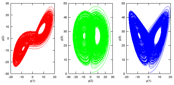
Figure 2. Solution of the Lorenz equations for P = 10, r = 28 and b = 8/3, from t = 0 to 250. Each projection shows two lobes, and the path switches between them at irregular times.

• The left plot is x against y : the two lobes lie along a diagonal, one in the lower left and one in the upper right. Near the lobe centers, x and y have the same sign.
• The middle plot is y against z : the lobes sit side by side between z = 0 and about 50, with holes near y = -8.5 and y = 8.5.
• The right plot is x against z : this is the familiar butterfly. The holes near x = +/-8.5 and z = 27 are the two unstable fixed points that the section on rho computes.
• A thin line enters from the bottom : the run starts at (1, 1, 1). The line near z = 1 in the middle and right plots is the path on its way to the attractor.

The Matlab code to get the solution to the equations and plot them is as follows :

%Save the following contents in a .m file and run the .m file

% this is tested only in Matlab, not in Octave

P = 10;

r = 28;

b = 8/3;

 

dy_dt = @(t,y) [-P*y(1)+P*y(2);...

                    r.*y(1)-y(2)-y(1)*y(3);...

                    y(1)*y(2)-b.*y(3)];

 

odeopt = odeset ('RelTol', 0.00001, 'AbsTol', 0.00001,'InitialStep',0.5,'MaxStep',0.5);

[t,y] = ode45(dy_dt,[0 250], [1.0 1.0 1.0],odeopt);

 

subplot(1,3,1);plot(y(:,1),y(:,2),'r-'); xlabel('y(1)'); ylabel('y(2)');

subplot(1,3,2);plot(y(:,2),y(:,3),'g-'); xlabel('y(2)'); ylabel('y(3)');

subplot(1,3,3);plot(y(:,1),y(:,3),'b-'); xlabel('y(1)'); ylabel('y(3)');

 

Let's match the listing to the equations. The state vector y holds x, y and z as y(1), y(2) and y(3). So -P*y(1)+P*y(2) is σ(y - x), r.*y(1)-y(2)-y(1)*y(3) is x(ρ - z) - y, and y(1)*y(2)-b.*y(3) is xy - βz. ode45 is an adaptive Runge-Kutta solver. The odeset line sets both tolerances to 0.00001 and limits every step to 0.5. The run covers t = 0 to 250 from the start point (1, 1, 1), and the three subplot lines draw the projections of Figure 2.

The program at the top of the page solves the same equations in a different way. It uses the classical fourth order Runge-Kutta method, RK4, with a fixed step equal to the Time Step value. It starts from (0.1, 0, 0) instead of (1, 1, 1). Its Beta field shows 2.67, but the program starts with the exact value 8/3. It switches to the value in the field only after you edit it. Because the system is chaotic, the two solvers give different paths after some time, while the shape of the attractor stays the same.

• Three equations, two nonlinear terms : xz and xy couple the variables, and without them the system could not be chaotic.
• Single variables look random, projections show structure : x(t) alone jumps between positive and negative runs, while any two variables together draw the two lobes.
• Different solvers give different paths but the same attractor : ode45 and the RK4 program disagree on the exact path after a while, and both fill the same butterfly.

What happens when rho changes ?

The butterfly appears only for some parameter values. With σ = 10 and β = 8/3 fixed, the value of ρ decides whether the fluid stays still, rolls steadily or becomes chaotic. The fixed points of the equations, and their stability, explain where each change happens.

A fixed point is a state where all three derivatives are zero. The origin (0, 0, 0) is always one. For ρ > 1, two more appear: C⁺ and C^- = (+/-√(β(ρ - 1)), +/-√(β(ρ - 1)), ρ - 1). The origin is the fluid at rest, and C⁺ and C^- are steady convection rolls that turn in opposite directions. For ρ = 28, the two points are (+/-8.49, +/-8.49, 27). These are the centers of the two lobes in Figure 2.

Each fixed point can attract or repel nearby paths. The origin attracts for ρ < 1 and repels for ρ > 1. C⁺ and C^- attract until ρ reaches ρ_H = σ(σ + β + 3) / (σ - β - 1). With σ = 10 and β = 8/3, this gives ρ_H = 24.74. Above that value, no fixed point attracts, and the path has nowhere to settle. The table below lists the three ranges, with end points from the RK4 method of the program.

Why does the path stay bounded when nothing attracts it ? The equations shrink every small volume of states. The divergence of the right side is -(σ + 1 + β), which is -13.67 for the classic values. So a small volume shrinks by a factor of e^-13.67, about 0.0000012, in every time unit. The paths therefore collapse onto a set with zero volume. That set is the strange attractor: a thin, layered surface with a fractal dimension a little above 2.

• Rho below 1 means no convection : every path decays to the origin.
• Rho between 1 and 24.74 means steady rolls : the path settles on C⁺ or C^-, depending on the start point.
• Rho above 24.74 means no stable fixed point : for ρ = 28 the path circles the two unstable points and switches lobes at irregular times.
• Volumes shrink but paths do not settle : the divergence of -13.67 squeezes the paths onto a thin attractor with zero volume.

How fast do two nearby paths separate ?

The introduction says that a minute change in the start values leads to a different outcome. Let's put a number on that claim. The number is the largest Lyapunov exponent, and it tells you how much prediction you gain from a better measurement.

Start two paths very close together on the attractor, and measure the distance d(t) between them. On average, the distance grows like d(t) = d(0) x e^λt. For σ = 10, ρ = 28 and β = 8/3, a numerical estimate with RK4 and a step of 0.01 gives λ = 0.906. So the distance grows by a factor of about 2.5 in each time unit, and it doubles in about 0.77 time units.

The program shows the same effect. Start one run from X0 = 0.1 and another from X0 = 0.101, a change of 0.001, and keep every other value at its default. The two paths stay within 5 units of each other until about t = 30. With a change of only 0.00000001, they stay together until about t = 45. So a start value that is 100000 times more accurate adds only about 15 time units of useful prediction. This is the logarithmic law that makes long-range weather forecasting hard.

The same law explains the Time Step effect in the program. A different step size changes the rounding and the truncation error in every step. That error acts like a small change in the start point, so runs with different steps separate after a while. Each run still traces the same attractor.

• Nearby paths separate like e^0.906t : the error grows by about 2.5 in every time unit.
• Better measurements buy little time : a 100000 times smaller start error adds only about 15 time units before the paths separate.
• The shape is predictable, the path is not : every start point and every step size fills the same attractor, but the position at a later time cannot be known.