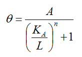
It is very usefull function to approximate various degree of Hard Limitor (Similar to Step function) just by changing Ka, A, n in the following equation. This is very widely used in BioChemistry.
Let's first read what each symbol in the equation does, and then plot the curve for a positive and a negative n. Every example keeps A = 0.5 and KA = 1.0, so all the curves share one point at L = 1. That shared point is the key to reading the plots.
- What does each parameter do ?
- How does a positive n shape the curve ?
- How does a negative n shape the curve ?
What does each parameter do ?
The equation has one input and three parameters. L is the input. In biochemistry it is the concentration of a ligand, a molecule that binds to a protein. θ is the output, the fraction of binding sites that are occupied. A is the upper limit of θ. Biochemistry uses A = 1, so θ runs from 0 to 1. The examples below use A = 0.5, which only scales the height of the curve.
KA sets where the switch happens. At L = KA the ratio KA/L is 1, so θ = A/(1 + 1) = A/2 for any n. In biochemistry KA is the ligand concentration that fills half of the sites. The code on this page writes it as Ka.
n is the Hill coefficient, and it sets how sharp the switch is. If you multiply the top and the bottom of the equation by Ln, you get the form that most textbooks use.
θ = A Ln / (KAn + Ln)
For n > 0, θ starts at 0 when L = 0 and rises toward A as L grows. For n = 0, (KA/L)0 is 1, so θ = A/2 for every L and the curve is a flat line. For n < 0, the curve is mirrored. It starts at A and falls toward 0.
The slope at the midpoint shows the effect of n directly. The derivative at L = KA is dθ/dL = nA/(4KA), so the slope there grows in proportion to n. As n goes to infinity, the curve becomes a step from 0 to A at L = KA. That step is the Hard Limitor of the introduction.
The input range of the switch gives another view of the sharpness. θ reaches 10% of A at L = KA/91/n and 90% of A at L = 91/nKA. The ratio between the two inputs is 811/n, and the table below lists it for a few values of n.
n |
L at 90% of A / L at 10% of A |
1 |
81 |
2 |
9 |
4 |
3 |
10 |
1.55 |
So with n = 1 the input has to grow 81 times to move θ from 10% to 90% of A. With n = 4 a factor of 3 is enough.
One more form is useful when you fit the curve to measured data. Rearranging the equation gives log(θ/(A - θ)) = n log L - n log KA. So a plot of log(θ/(A - θ)) against log L is a straight line. Its slope is n, and it crosses zero at L = KA. Biochemists call this the Hill plot.
KA is the midpoint : θ = A/2 at L = KA, whatever the value of n.n sets the steepness : The slope at the midpoint is nA/(4KA), and the 10% to 90% input range is a factor of 811/n.The sign of n sets the direction : A positive n gives a rising curve, a negative n a falling curve, and n = 0 a flat line at A/2.A only scales the height : It changes the upper limit of θ and nothing else.
How does a positive n shape the curve ?
Let's now look at the curve for a positive n. The examples keep A = 0.5 and KA = 1.0 and sweep L from 0 to 10, so n is the only thing that changes. The first example plots one curve, and the second overlays eleven of them.
Example 1 - When n >= 0
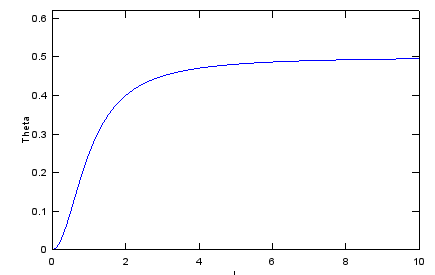
Example 1 fixes n = 2. Before looking at the plot, use the previous section to predict three points. The curve starts at 0, passes 0.25 at L = 1, and approaches A = 0.5 for a large L.
n = 2;
A = 0.5;
Ka = 1.0;
L = 0:0.1:10;
Theta = A ./((Ka ./ L).^n .+ 1);
plot(L,Theta); xlim([L(1),L(length(L))]); ylim([0,1.25 .* max(Theta)]);xlabel('L');ylabel('Theta');
The plot matches all three points. At L = 2 the formula gives 0.5/(0.25 + 1) = 0.4, which is also where the curve sits. The curve starts flat near L = 0. This happens for every n > 1, and it gives the S shape, or sigmoid, that makes the function a switch. With n = 1 the curve would instead start with its steepest slope.
The listing is Octave code. The operator .+ is an Octave-only form of +. MATLAB does not accept it, and newer Octave releases have dropped it too, so write a plain + there. At L = 0 the term Ka ./ L is Inf, and Inf plus 1 is still Inf, so the first value of Theta is 0 without any error.
Example 2 - When n >= 0
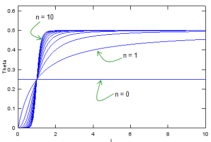
Example 2 draws n = 0, 1, 2 and so on up to 10 on the same axes. A and KA stay the same in every curve, so the plot shows the effect of n alone.
A = 0.5;
Ka = 1.0;
L = 0:0.1:10;
for n=0:1.0:10
Theta = A ./((Ka ./ L).^n .+ 1);
plot(L,Theta); xlim([L(1),L(length(L))]); ylim([0,1.25 .* max(Theta)]);xlabel('L');ylabel('Theta');
hold on;
end;
All eleven curves cross at L = 1, θ = 0.25, as the midpoint rule predicts. The n = 0 curve is the flat line at 0.25. The n = 1 curve rises quickly at first and then slowly, without an S shape. From n = 2 upward, each curve is steeper at L = 1 than the one before. The n = 10 curve is close to a step from 0 to 0.5, and that is how the function approximates a Hard Limitor.
Every curve passes through L = KA, θ = A/2 : Changing n rotates the curve around this point.n greater than 1 gives the S shape : The curve starts flat, which is what makes it act like a switch rather than a gradual rise.A large n approaches a step : At n = 10 the 10% to 90% range is only a factor of 1.55 in L.
How does a negative n shape the curve ?
A negative n turns the switch around. With n < 0, (KA/L)n equals (L/KA)|n|, so θ = A/(1 + (L/KA)|n|). The output is high for a small L and low for a large L. Biology uses this falling form for a repressor, where more input means less output.
The two cases are mirror images of each other. For the same L, the value for -n is A minus the value for n. So everything the previous section said about the midpoint and the steepness still holds, with the direction reversed.
Example 3 - When n <= 0
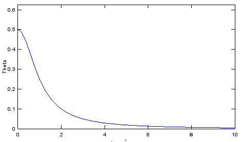
Example 3 repeats Example 1 with n = -2. By the mirror rule, each value should be 0.5 minus the Example 1 value at the same L.
n = -2;
A = 0.5;
Ka = 1.0;
L = 0:0.1:10;
Theta = A ./((Ka ./ L).^n .+ 1);
plot(L,Theta); xlim([L(1),L(length(L))]); ylim([0,1.25 .* max(Theta)]);xlabel('L');ylabel('Theta');
The curve starts at A = 0.5 when L = 0, and it passes 0.25 at L = 1 again. At L = 2 it gives 0.5/(1 + 4) = 0.1. That is 0.5 - 0.4, the mirror of the Example 1 value.
Example 4 - When n <= 0
Example 4 sweeps n = 0, -1, -2 and so on down to -10 on one plot. It is the mirror of Example 2, so compare the two plots side by side.
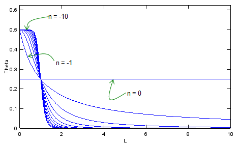
A = 0.5;
Ka = 1.0;
L = 0:0.1:10;
for n=0:-1.0:-10
Theta = A ./((Ka ./ L).^n .+ 1);
plot(L,Theta); xlim([L(1),L(length(L))]); ylim([0,1.25 .* max(Theta)]);xlabel('L');ylabel('Theta');
hold on;
end;
The curves again cross at L = 1, θ = 0.25. The n = -1 curve falls slowly, and the n = -10 curve is close to a step down from 0.5 to 0. So a large negative n approximates an inverted Hard Limitor.
The value for -n is A minus the value for n : A negative n mirrors the positive case around the line θ = A/2.A negative n gives a falling switch : The output starts at A and drops to 0 as L grows past KA.The midpoint and the steepness do not change : Only the direction flips, so |n| still sets how sharp the step is.