In the above section, you saw some examples of how a matrix can transform a shape in a coordinate. But all the elements in the matrix and the numbers representing a point in a coordinate were real numbers.

In this section,  you would see examples where complex numbers are used in both matrix and coordinate. As you may see in complex number section, the operation of the complex number itself has some geometric transformation properties. Therefore, the final outcome of the transformation of complex coordinate and complex matrix are even more complicated. Only real practice on your own would give you the real meaning of those transformation.

This kind of transformation are used pretty often in MIMO (Multiple Input Multiple Output) in wireless communication.

On this page, a 2 x 2 complex matrix takes two constellation points and returns two new ones. I'll first set up the code, then run four examples with different input pairs. The last section shows what the three matrices share, and why they are exactly the 2-layer precoders of the LTE 2-antenna codebook.

• How is the example code set up ?
• What happens when c1 = v1 and c2 = v2 ?
• What happens when c1 = v1 and c2 = v3 ?
• What happens when c1 = v1 and c2 = v4 ?
• What happens when c1 = v1 and c2 = v1 ?
• What do the three matrices have in common ?
• Reference

How is the example code set up ?

Let's directly jump into some examples. Following is a Matlab/Octave code that I wrote. v1, v2, v3, v4 are a complex number representing a constellation point in I/Q coordinate. m1,m2,m3 is a complex transformation matrix. c1, c2 can be any two complex numbers selected from {v1, v2, v3, v4}.

Just try this code and observe the result. Change any of v1,v2,v3,v4, c1,c2, m1,m2,m3 and rerun the code. Repeat this process until your brain get the overall pictures of how this transformation work.

v1 = 1 + j;
v2 = -1 + j;
v3 = -1 - j;
v4 = 1 - j;

c1 = v1;
c2 = v2;

m1 = 1/sqrt(2).*[1 0; 0 1]
m2 = 1/2.*[1 1; 1 -1]
m3 = 1/2.*[1 1; j -j]

m1_c12 = m1 * [c1;c2]
m2_c12 = m2 * [c1;c2]
m3_c12 = m3 * [c1;c2]

subplot(2,2,1);
plot(real(v1), imag(v1),'ro','MarkerFaceColor',[1 0 0], 'MarkerSize',10, ...
     real(v2), imag(v2),'go','MarkerFaceColor',[0 1 0], 'MarkerSize',10, ...
     real(v3), imag(v3),'bo','MarkerFaceColor',[0 0 1], 'MarkerSize',10, ...
     real(v4), imag(v4),'yo','MarkerFaceColor',[1 1 0], 'MarkerSize',10);
     axis([-1.5 1.5 -1.5 1.5]);
     title('A');

subplot(2,2,2);
plot(real(c1), imag(c1),'ro','MarkerFaceColor',[1 0 0], 'MarkerSize',10, ...
     real(c2), imag(c2),'go','MarkerFaceColor',[0 1 0], 'MarkerSize',10, ...
     real(m1_c12), imag(m1_c12),'ko','MarkerFaceColor',[0 0 0], 'MarkerSize',10);
     axis([-1.5 1.5 -1.5 1.5]);
     title('B = m1 * [c1;c2]');

subplot(2,2,3);
plot(real(c1), imag(c1),'ro','MarkerFaceColor',[1 0 0], 'MarkerSize',10, ...
     real(c2), imag(c2),'go','MarkerFaceColor',[0 1 0], 'MarkerSize',10, ...
     real(m2_c12), imag(m2_c12),'ko','MarkerFaceColor',[0 0 0], 'MarkerSize',10);
     axis([-1.5 1.5 -1.5 1.5]);
     title('C = m2 * [c1;c2]');

subplot(2,2,4);
plot(real(c1), imag(c1),'ro','MarkerFaceColor',[1 0 0], 'MarkerSize',10, ...
     real(c2), imag(c2),'go','MarkerFaceColor',[0 1 0], 'MarkerSize',10, ...
     real(m3_c12), imag(m3_c12),'ko','MarkerFaceColor',[0 0 0], 'MarkerSize',10);
     axis([-1.5 1.5 -1.5 1.5]);
     title('D = m3 * [c1;c2]');

The four points v1 to v4 are the QPSK constellation, 1 + j, -1 + j, -1 - j and 1 - j, before any power normalization. Each matrix multiplies the column vector [c1; c2], so each one turns a pair of points into a new pair. Every output is a combination of both inputs, not a transformation of one point on its own.

Watch the colors when you read the plots. Graph A uses the legend under each example: red for v1, green for v2, blue for v3 and yellow for v4. Graphs B, C and D, however, always plot c1 in red and c2 in green, whichever points c1 and c2 are. So in the examples below, the green dot in B, C and D is c2, even when c2 is v3, v4 or v1. A later dot also hides an earlier dot at the same position, and the black outputs are drawn last.

• The input is a pair of points : the matrix acts on the vector [c1; c2], so both points change together.
• m1 only scales : it multiplies each point by 1/√2 = 0.70711 and keeps its angle.
• m2 and m3 mix the two points : their first row forms a sum and their second row forms a difference.

What happens when c1 = v1 and c2 = v2 ?

As the first example, I selected v1 and v2 as the two numbers to be transformed by the matrix. Following is the numerical result of the transformation. m1_c12 is the result of transformation of (c1,c2) by the matrix m1. m2_c12 is the result of transformation of (c1,c2) by the matrix m2. m3_c12 is the result of transformation of (c1,c2) by the matrix m3.

c1 = v1;
c2 = v2;

m1_c12 =

   0.70711 + 0.70711i
  -0.70711 + 0.70711i

m2_c12 =

   0 + 1i
   1 + 0i

m3_c12 =

   0 + 1i
   0 + 1i

Following is the graphical representation of the result of this transformation. Graph A shows the four complex numbers v1,v2,v3,v4 in I/Q coordinate.

Red = v1

Green = v2

Blue = v3

Yellow = v4

Black = the result of transformation of (c1,c2) by m1, m2, m3

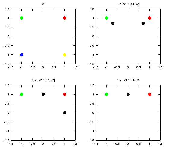
Figure 1. Input pair c1 = v1 and c2 = v2. m1 pulls both points toward the origin, m2 gives j and 1, and m3 puts both outputs on j.

Let's check the three results by hand. The matrix m1 only scales, so the black dots in plot B are c1 and c2 moved toward the origin by the factor 0.70711. The matrix m2 forms the sum and the difference of the two inputs. Its outputs are (c1 + c2)/2 = (2j)/2 = j and (c1 - c2)/2 = 2/2 = 1, which are the black dots in plot C. The matrix m3 has the same first row, so its first output is also j. Its second row gives j(c1 - c2)/2 = j x 1 = j. So both outputs of m3 fall on the same point, and plot D shows only one black dot.

• A sum and a difference : m2 and m3 both output (c1 + c2)/2 first. They differ only in how they present the difference.
• m3 turns the difference by 90 deg : its second row multiplies (c1 - c2)/2 by j.
• Two outputs can coincide : in plot D, both outputs of m3 equal j.

What happens when c1 = v1 and c2 = v3 ?

In the second example, I selected v1 and v3 as the two numbers to be transformed by the matrix. Following is the numerical result of the transformation. m1_c12 is the result of transformation of (c1,c2) by the matrix m1. m2_c12 is the result of transformation of (c1,c2) by the matrix m2. m3_c12 is the result of transformation of (c1,c2) by the matrix m3.

c1 = v1;
c2 = v3;

m1_c12 =

   0.70711 + 0.70711i
  -0.70711 - 0.70711i

m2_c12 =

   0 + 0i
   1 + 1i

m3_c12 =

   0 + 0i
  -1 + 1i

Following is the graphical representation of the result of this transformation. Graph A shows the four complex numbers v1,v2,v3,v4 in I/Q coordinate.

Red = v1

Green = v2

Blue = v3

Yellow = v4

Black = the result of transformation of (c1,c2) by m1, m2, m3

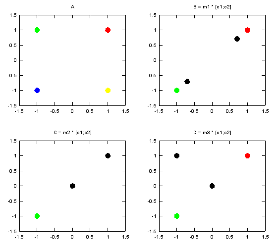
Figure 2. Input pair c1 = v1 and c2 = v3 = -v1. The sum is zero, so m2 and m3 put their first output at the origin.

Here c2 is exactly -c1, so the sum c1 + c2 is 0. That is why m2 and m3 both put their first output at 0 + 0i. The difference c1 - c2 = 2c1 now carries all the energy. The matrix m2 returns (c1 - c2)/2 = c1 = 1 + 1i, and m3 returns j c1 = -1 + 1i, which is c1 turned by 90 deg. In plot C, the black dot at 1 + 1i covers the red dot of c1. The green dot in plots B to D is c2 = v3 at -1 - 1i, although the legend lists v3 as blue.

• Opposite inputs cancel in the sum : the first output of m2 and m3 is 0 whenever c2 = -c1.
• The difference keeps the energy : the second output holds c1, or c1 turned by 90 deg for m3.
• m1 keeps the points opposite : 0.70711 + 0.70711i and -0.70711 - 0.70711i are still mirror images through the origin.

What happens when c1 = v1 and c2 = v4 ?

In the third example, I selected v1 and v4 as the two numbers to be transformed by the matrix. Following is the numerical result of the transformation. m1_c12 is the result of transformation of (c1,c2) by the matrix m1. m2_c12 is the result of transformation of (c1,c2) by the matrix m2. m3_c12 is the result of transformation of (c1,c2) by the matrix m3.

c1 = v1;
c2 = v4;

m1_c12 =

   0.70711 + 0.70711i
   0.70711 - 0.70711i

m2_c12 =

   1 + 0i
   0 + 1i

m3_c12 =

   1
  -1

Following is the graphical representation of the result of this transformation. Graph A shows the four complex numbers v1,v2,v3,v4 in I/Q coordinate.

Red = v1

Green = v2

Blue = v3

Yellow = v4

Black = the result of transformation of (c1,c2) by m1, m2, m3

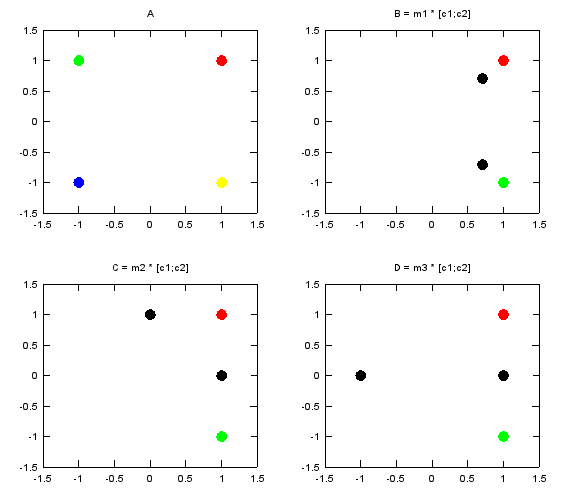
Figure 3. Input pair c1 = v1 and c2 = v4, the complex conjugate of v1. All outputs of m2 and m3 fall on the real or the imaginary axis.

In this pair, c2 is the complex conjugate of c1. Their sum, 2, is purely real, and their difference, 2j, is purely imaginary. So m2 returns 1 and j. The matrix m3 multiplies the difference by j once more, and j x j = -1. So its outputs are 1 and -1, both on the real axis, as plot D shows. The output m3_c12 is printed as 1 and -1 without an imaginary part, because both values are real.

• Conjugate inputs give a real sum : the sum of a number and its conjugate is twice its real part.
• The difference is imaginary : it is twice the imaginary part, times j.
• m3 can make the output fully real : its extra factor j turns the imaginary difference back onto the real axis.

What happens when c1 = v1 and c2 = v1 ?

In the fourth example, I selected v1 and v1 again as the two numbers to be transformed by the matrix. Following is the numerical result of the transformation. m1_c12 is the result of transformation of (c1,c2) by the matrix m1. m2_c12 is the result of transformation of (c1,c2) by the matrix m2. m3_c12 is the result of transformation of (c1,c2) by the matrix m3.

c1 = v1;
c2 = v1;

m1_c12 =

   0.70711 + 0.70711i
   0.70711 + 0.70711i

m2_c12 =

   1 + 1i
   0 + 0i

m3_c12 =

   1 + 1i
   0 + 0i

Following is the graphical representation of the result of this transformation. Graph A shows the four complex numbers v1,v2,v3,v4 in I/Q coordinate.

Red = v1

Green = v2

Blue = v3

Yellow = v4

Black = the result of transformation of (c1,c2) by m1, m2, m3

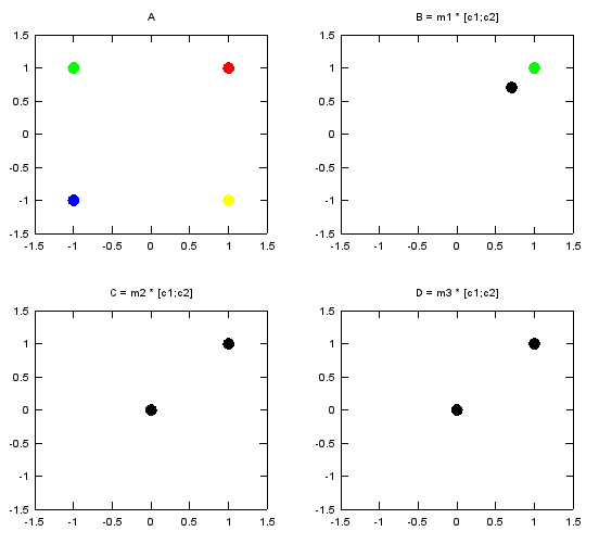
Figure 4. Input pair c1 = c2 = v1. The difference is zero, so m2 and m3 put their second output at the origin.

With two equal inputs, the difference c1 - c2 is 0. So the second output of both m2 and m3 is 0 + 0i. The sum 2c1 gives the first output c1 = 1 + 1i for both matrices, and m3 cannot be told apart from m2 in this case. In plot B, the green dot of c2 covers the red dot of c1, because the two points are the same. The two outputs of m1 also coincide at 0.70711 + 0.70711i.

• Equal inputs cancel in the difference : the second output of m2 and m3 is 0 whenever c2 = c1.
• m2 and m3 agree when the difference is 0 : they differ only in the second row.
• Coinciding dots hide each other : count the entries of the printed output, not the dots in the plot.

What do the three matrices have in common ?

The four examples look different, but the three matrices follow one pattern. Each one keeps the total power of the pair in a fixed ratio, and each one can be undone. These two properties are what a MIMO transmitter needs from a precoder.

Let's start with the power. In every example, the input pair has |c1|² + |c2|² = 2 + 2 = 4. Every output pair of m1, m2 and m3 has a total power of 2. So each matrix halves the power of the pair, whatever the input. The reason is that √2 m1, √2 m2 and √2 m3 are unitary matrices. Their columns are orthogonal and have unit length, so they rotate the pair without changing its power. The factor 1/√2 then scales the power by 1/2.

Next, the inverse. Each matrix has one, so a receiver can recover c1 and c2 from the two outputs. The inverse of m2 is [1 1; 1 -1], and the inverse of m3 is [1 -j; 1 j]. Both equal 2 times the conjugate transpose of the matrix, which is the unitary property again. For example, the outputs j and 1 of the first example give back [1 1; 1 -1] x [j; 1] = [1 + j; -1 + j], which is the input pair v1 and v2.

The three matrices are not arbitrary. The table below is the codebook for transmission on two antenna ports in 36.211 Table 6.3.4.2.3-1. Its 2-layer column holds m1, m2 and m3 of the code above, as codebook index 0, 1 and 2. For closed-loop spatial multiplexing with two layers, 36.211 does not use codebook index 0, so an LTE UE chooses between m2 and m3 in its PMI report.

The scale factors 1/√2 and 1/2 normalize the transmit power. With unit-power layer symbols, the total power over the two antenna ports is 1, for one layer and for two layers alike. In the examples above, the QPSK points were not normalized, so the totals were 4 in and 2 out instead.

• Each matrix is a scaled unitary matrix : it rotates the pair of points in two complex dimensions, and then scales it by 1/√2.
• The total power halves : every example goes from 4 to 2, whatever the input pair.
• A receiver can undo each matrix : the inverse is 2 times the conjugate transpose.
• m1, m2 and m3 are the LTE 2-layer precoders : they are codebook index 0, 1 and 2 of 36.211 Table 6.3.4.2.3-1.

Reference

The codebook table in the previous section was checked against the specification listed below.

• 3GPP TS 36.211 v19.3.0, Evolved Universal Terrestrial Radio Access - Physical channels and modulation, Table 6.3.4.2.3-1