LU decomposition is a method to split (decompose) a matrix into two matrix product. One of these two matrix(the first part) is called 'L' matrix meaning 'Lower triangular matrix' and the other matrix(the second part) is called 'U' matrix meaning 'Upper triangular matrix'. Simply put, LU decomposition is a process to convert a Matrix A into the product of L and U as shown below.

A = LU

A lower triangular matrix is a matrix where all the elements above the main diagonal (top left to bottom right) are zero. An upper triangular matrix is a matrix where all the elements below the main diagonal are zero.

I would not explain about how you can decompose a matrix into LU form. The answer is "Use software" -:). I would talk about WHY.

• How L and U is applied ?
• Application of LU Decomposition
• Beneifit vs Overhead
• Size Matters ?
• Restrictions or Limitations ?
• Alternative methods and advantage over LU decomposition

How L and U is applied ?

In this section I want to show you an example of how the LU decomposed matrix is applied for a case of solving a linear equation (a linear simultaneous equation)

LU decomposition is used to solve a system of linear equations by factoring a square matrix A into a lower triangular matrix L and an upper triangular matrix U. Given a system of linear equations in the form Ax = b, where A is a square matrix, x is the column vector of unknowns, and b is the column vector of constants, the LU decomposition allows us to solve this system more efficiently.

By breaking down the original system of linear equations into two triangular systems and solving them with forward and back substitution, the LU decomposition allows us to solve the system of simultaneous linear equations efficiently. This method is particularly useful when dealing with large systems of linear equations or when solving multiple systems with the same coefficient matrix A but different constant vectors b.

Here's how the LU decomposition can be applied for solving a system of simultaneous linear equations:

Step 1: Decompose the matrix A into L and U

Perform the LU decomposition to factor the given square matrix A into a lower triangular matrix L and an upper triangular matrix U, such that A = LU.

Step 2: Solve for an intermediate vector y using forward substitution:

Since A = LU, we can rewrite the system of equations as LUx = b. Now, let Ux = y. This gives us the new system of equations Ly = b.

Because L is a lower triangular matrix, we can use forward substitution to solve for y. Start with the first row of L and solve for y1, then move to the second row and solve for y2, and so on until you reach the last row and solve for yn. This process is computationally efficient, as each row needs only one division, plus one multiplication for each value already found.

Step 3: Solve for the unknown vector x using back substitution:

Now that we have the intermediate vector y, we can solve the system Ux = y for the unknown vector x. Since U is an upper triangular matrix, we can use back substitution to solve for x. Start with the last row of U and solve for xn, then move to the second-to-last row and solve for xn-1, and so on until you reach the first row and solve for x1. This process is also computationally efficient, as each row needs only one division, plus one multiplication for each value already found.

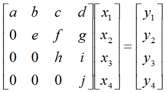
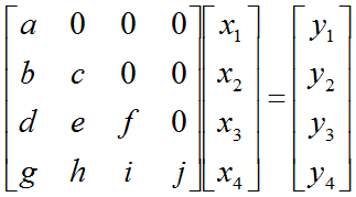
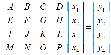
Let's assume that we have a matrix equation (Linear Equation) as shown below.

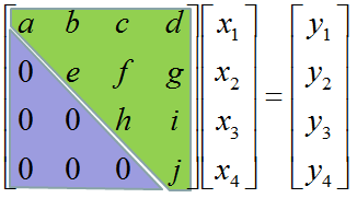
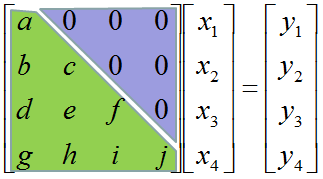
Don't look into each elements yet. Just get around 100 steps back away from this and look at the overall pattern of the matrix. Can you see a pattern as shown below ? You see two area marked as triangles. Green triangle shows all the elements from diagonal line and upper diagonal part. The elements in this triangle is non-zero values. Violet triangle shows the elements of lower diagonal part which is all zero.

This form of matrix is called 'U' form matrix, meaning 'Upper triangular matrix'. Why this is so special ?

It is special because it is so easy to solve the equation.  Now let's think about how we can solve this equation.

Let's look the last row (4th row in this case). How can I figure out the value for x4 ? You would get it right away because there is only x4 term and j and y4 are known values.

Once you get x4 and plug in the x4 value into row 3, then you would get x3 value.

Once you get x3 and plug in the x3 value into row 2, then you would get x2 value.

Once you get x2 and plug in the x2 value into row 1, then you would get x1 value.

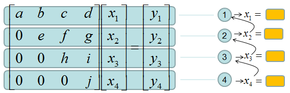
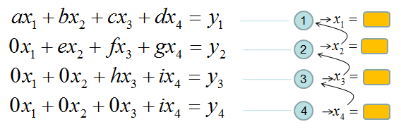
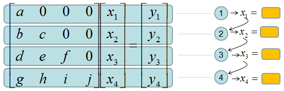
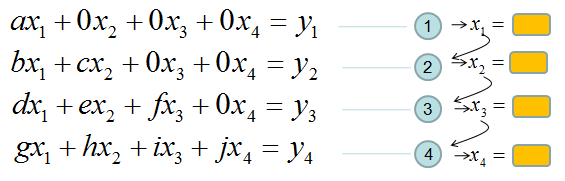
If it is not clear with you, it would be a little clearer if you convert the matrix equation into simultaneous equation as shown below.  

Start from the last equation and get x4 first and repeat the process described above.

One slip in the picture above needs a correction. The last equation should read 0x₁ + 0x₂ + 0x₃ + jx₄ = y₄, because the element in row 4 and column 4 of the matrix is j, not i. So the first step is x₄ = y₄ / j.

If this process is still unclear,just play with real numbers. Put any numbers for a,b,c,d,e,f,g,h,i,j,y1,y2,y3,y4 and try to get x1,x2,x3,x4 as explained above.

If you tried this as explained, one thing you would notice would be "It is so simple to find the solution x1,x2,x3,x4". Just compare this process with what you experienced with general matrix equation solving process you did in your high school math or linear algebra class.

Now let's look into another example of matrix equation as shown below.

Now you would know what I will say. In this case, all the elements along the diagonal line and Lower part of diagonal line is non-zero values. All the values above the diagonal line is all zero.

This form is called 'L' form meaning 'Lower triangular matrix'.

Why this is so special ?

It is special because it is so easy to solve the equation.  Now let's think about how we can solve this equation.

Let's look the first row (the first row in this case). How can I figure out the value for x1 ? You would get it right away because there is only x1 term and a and y1 are known values.

Once you get x1 and plug in the x1 value into row 2, then you would get x2 value.

Once you get x2 and plug in the x2 value into row 3, then you would get x3 value.

Once you get x3 and plug in the x3 value into row 4, then you would get x4 value.

If it is not clear with you, it would be a little clearer if you convert the matrix equation into simultaneous equation as shown below.  

Start from the first equation and get x1 first and repeat the process described above.

If this process is still unclear,just play with real numbers. Put any numbers for a,b,c,d,e,f,g,h,i,j,y1,y2,y3,y4 and try to get x1,x2,x3,x4 as explained above.

If you tried this as explained, one thing you would notice would be "It is so simple to find the solution x1,x2,x3,x4". Just compare this process with what you experienced with general matrix equation solving process you did in your high school math or linear algebra class.

Now let's suppose we have a matrix as shown below. Here all the elements in the matrix is non-zero values.

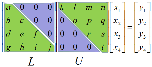
Now let's assume we can convert this matrix equation into following form. (Don't worry about HOW, just assume you can do this somehow). You already know that this form would make it easier to solve the equation.

Let's connect the L and U diagram above with Steps 1 to 3. The diagram calls the right-hand side y, while the steps call it b and use y for the intermediate vector. With the names of the steps, you first solve L(Ux) = b for the vector Ux with forward substitution, as in the L example. Then you solve U x = (that vector) with back substitution, as in the U example. Each stage is one of the easy triangular problems you just worked through.

One more detail matters when you compare your own result with software. In the diagram, L has a, c, f and j on its diagonal, and U has k, o, r and t. You can move a scale factor from one matrix to the other without changing the product LU. So the decomposition is not unique until you fix this freedom. Most software, including Matlab, returns an L with 1 on every diagonal element.

Try this example that I found from web. (If the link is missing, try here).

Now you may say.. "You always say 'don't worry about how to solve. just use computer software'". If I use the computer software, why do I have to worry about this kind of conversion. Computer software would not have any problem to solve the equation even with the original form without LU decomposition.

You are right, the computer program would not have any problem with original form. But the amount of time for the calculation is much shorter with LU decomposed form than doing the same thing in the original form. When the size of matrix is small, this time difference would be negligiable, but if the size is very huge (e.g, 10000 x 10000) the time difference would be very huge. If you've done a computer science, you would be familiar with Big O notation to evaluate the computation time. Try compare the computation time for the original matrix form and LU decomposed form. If you are not familiar with this notation, just trust me -:).

Following two YouTube tutorial would give you some insight of LU decomposition including computation time.

• LU Decomposition Method : Basis
• LU Decomposition: Why Part 2 of 2

A worked example with numbers

The letters above show the pattern, but numbers show the work. Let's take a 3 x 3 system, factor it by hand, and then run the two substitutions. Every value below can be checked with a pen, and the result agrees with Matlab.

A = [ 2  1  1 ;  4 -6  0 ; -2  7  2 ]        b = [ 5 ; -2 ; 9 ]

L = [ 1  0  0 ;  2  1  0 ; -1 -1  1 ]        U = [ 2  1  1 ;  0 -8 -2 ;  0  0  1 ]

Forward substitution, L y = b :   y1 = 5
                                  y2 = -2 - 2 x 5            = -12
                                  y3 = 9 + 5 + (-12)         = 2

Back substitution, U x = y :      x3 = 2 / 1                 = 2
                                  x2 = (-12 + 2 x 2) / (-8)  = 1
                                  x1 = (5 - 1 - 2) / 2       = 1

The entries of L are the multipliers of Gaussian elimination. To clear the 4 under the first pivot 2, you subtract 2 times row 1, so L has 2 in row 2 and column 1. To clear the -2, you subtract -1 times row 1, so L has -1 in row 3. After that step, row 3 reads [0 8 3], and you subtract -1 times the new row 2, which gives the last -1. U is simply the matrix that is left when elimination ends.

If you run [L,U,P] = lu(A) in Matlab, the output will look different. Matlab uses partial pivoting and picks 4 as the first pivot, because 4 is the largest value in the first column. It returns P = [0 1 0; 1 0 0; 0 0 1], L = [1 0 0; 0.5 1 0; -0.5 1 1] and U = [4 -6 0; 0 4 1; 0 0 1], so that P*A = L*U. Both factorizations are correct, and both give x = [1; 1; 2].

• L records the elimination steps and U is the result : you get both from the same Gaussian elimination, with no extra work.
• Each substitution is one pass over a triangle : forward substitution runs from the top row down, and back substitution runs from the bottom row up.
• Software output can differ from a hand calculation : row exchanges and the choice of 1 on the diagonal of L change the factors, but not the solution.

Application of LU Decomposition

Once you have L and U, they are not tied to a single right-hand side. Every job in this section reuses the same two triangular matrices, and that reuse is where the saving comes from. Let's go through the jobs one at a time.

LU decomposition has several applications in various fields, such as engineering, computer science, physics, and economics. Some common applications include:

Solving systems of linear equations:

A system of linear equations can be represented as Ax = b, where A is a matrix, x is a column vector of unknowns, and b is a column vector of constants. LU decomposition can simplify solving such systems by breaking down matrix A into L and U. Once we have the LU decomposition, we can solve the system in two steps:

a) Forward substitution: Solve Ly = b for y.

b) Back substitution: Solve Ux = y for x.

The advantage of this approach is that triangular matrices are much easier to work with when solving linear systems compared to the original matrix A.

Computing determinants:

Finding the determinant of a matrix is an important operation in linear algebra. Once a matrix A is decomposed into L and U, the determinant of A can be found as the product of the diagonal elements of L and U. This is because the determinant of a triangular matrix is equal to the product of its diagonal elements, and det(A) = det(L) * det(U).

Finding matrix inverses:

The inverse of a matrix A, denoted A^(-1), is used to solve systems of linear equations and perform various calculations. Using LU decomposition, we can efficiently compute the inverse of A. If A = LU, then A^(-1) = U^(-1) * L^(-1). We can find the inverse of L and U separately using forward and back substitution and then multiply them to obtain A^(-1).

Numerical stability and efficiency:

In certain cases, the LU decomposition with partial pivoting can help improve the numerical stability of calculations. Partial pivoting involves reordering the rows of the matrix A to ensure that the largest element (in absolute value) in each column is on the diagonal. This can help reduce the effects of round-off errors and improve the accuracy of calculations.

Eigenvalue and eigenvector computations:

In some algorithms for finding eigenvalues and eigenvectors of a matrix, LU decomposition is used as an intermediate step. These algorithms, such as inverse iteration, can benefit from the efficiency and numerical stability provided by LU decomposition.

Let's put numbers on two of these jobs with the worked example above. The determinant is the product of the diagonal of U, because the diagonal of L holds only 1s. So det(A) = 2 x (-8) x 1 = -16. With the pivoted Matlab factors, the product of the diagonal of U is 4 x 4 x 1 = 16. One row exchange flips the sign, so the result is again -16. In general, det(A) = (-1)^s x u₁₁u₂₂...u_nn, where s is the number of row exchanges.

For the inverse, you solve A x = e_k once for each column e_k of the identity matrix, using the same L and U every time. For the example, e₁ = [1; 0; 0] gives [0.75; 0.5; -1], which is the first column of A^-1. Keep in mind that you rarely need the inverse itself. To solve Ax = b, the two substitutions are cheaper and more accurate than computing A^-1 first and then multiplying it by b.

• The determinant comes almost for free : multiply the diagonal of U and correct the sign for each row exchange.
• An inverse is n solves with one factorization : each column of A^-1 needs one forward and one back substitution.
• Solve rather than invert : x = U\(L\b) is cheaper and more accurate than inv(A)*b.

Beneifit vs Overhead

I understand that it would be beneficial to use in various way once we have L and U components of a matrix. But doesn't it take time and effort to decompose a matrix into L and U components ? How would you compare the benefit with overhead ?

Good point.  There is a computational cost associated with decomposing a matrix into its L and U components. The process of LU decomposition generally involves Gaussian elimination or similar algorithms, which have a time complexity of O(n^3) for an n x n matrix. This means that as the size of the matrix grows, the time required to perform the decomposition increases significantly.

The benefits of using LU decomposition depend on the specific problem and the size of the matrices involved. For small matrices or one-time calculations, the overhead of LU decomposition might not be justifiable. However, for larger matrices or cases where the decomposition can be reused for multiple calculations, the benefits can outweigh the overhead, making LU decomposition a valuable tool in linear algebra.

However, the benefits of LU decomposition often outweigh the overhead, especially when solving large systems of linear equations, calculating determinants, or finding matrix inverses. Here's why:

Reusability: Once a matrix A is decomposed into L and U, the decomposition can be reused for solving multiple linear systems with the same matrix A but different right-hand side vectors (b). In such cases, the time spent on LU decomposition is a one-time cost, and subsequent linear system solutions become much faster using forward and back substitution.

Efficiency: When solving a linear system with LU decomposition, triangular matrices (L and U) are significantly easier to work with than the original matrix A. Forward and back substitution methods used for solving triangular systems have a time complexity of O(n^2), which is more efficient than solving the original system directly using methods like Gaussian elimination.

Numerical stability: In certain cases, LU decomposition with partial pivoting can help improve the numerical stability of calculations, reducing the effects of round-off errors and improving the accuracy of results.

There is an important detail behind this comparison. LU decomposition is not extra work on top of Gaussian elimination. Elimination on A already produces U, and the multipliers that it uses are the entries of L, as the worked example above shows. So for one system, LU costs the same as elimination. That is about 2n³/3 floating point operations, or flops. Each additional right-hand side then costs only about 2n² flops, n² for each substitution. The numbers below show how the gap grows with n.

n          LU factorization, 2n3/3      two substitutions, 2n2      ratio
100        6.7 x 105                    2.0 x 104                      33
1000       6.7 x 108                    2.0 x 106                      333
10000      6.7 x 1011                   2.0 x 108                      3333

This is also what Matlab does. For a general square matrix, x = A\b runs an LU factorization with partial pivoting and then the two substitutions. When you have many right-hand sides that arrive one at a time, factor once with [L,U,P] = lu(A). Then solve each new b with x = U\(L\(P*b)).

• LU is Gaussian elimination with the multipliers kept : factoring costs nothing beyond what solving one system already costs.
• The expensive part is done once : the factorization is O(n³), and every later solve is only O(n²).
• The saving grows with n : for n = 1000, one extra solve is about 333 times cheaper than a new factorization.

Size Matters ?

The real choice here is not whether to factor, because a dense direct solver always factors. The choice is between a dense LU and a method that never forms L and U at all. Size matters for that choice, but sparsity and memory usually matter more.

Is there any rule of thumb in terms of a threshold of a matrix size with the cost outweighing the benefit ?

Good Question.

There isn't a universal rule of thumb for a threshold matrix size where the benefits of LU decomposition consistently outweigh the costs, as the trade-offs depend on the specific problem and computational resources available. However, some general guidelines can be helpful when deciding whether to use LU decomposition:

Small matrices: For very small matrices (e.g., 2x2 or 3x3), the overhead of LU decomposition might not provide significant benefits, as direct methods like Gaussian elimination or Cramer's rule can efficiently solve linear systems or calculate determinants and inverses.

Reusability: If you need to solve multiple linear systems with the same matrix A but different right-hand side vectors (b), LU decomposition becomes more advantageous. The decomposition is a one-time cost, and solving subsequent linear systems using forward and back substitution is faster. In such cases, even for moderately sized matrices (e.g., 10x10), LU decomposition can be beneficial.

Large matrices: As the size of the matrix grows, the computational cost of LU decomposition and direct methods like Gaussian elimination both increase. However, the benefits of using LU decomposition may become more pronounced, particularly for solving linear systems, due to the efficiency of forward and back substitution with triangular matrices. For matrices larger than 100x100, iterative methods like the Conjugate Gradient method or GMRES may be more suitable, depending on the properties of the matrix.

Numerical stability: If the problem you're working on requires high numerical stability or involves ill-conditioned matrices, LU decomposition with partial pivoting can be a better option than direct methods, even for moderate-sized matrices.

Computational resources: The available computational resources (e.g., memory, processing power) can also influence the decision to use LU decomposition. For limited-resource environments, the benefits of LU decomposition might be more pronounced due to its efficient handling of large matrices.

Let's put numbers on the size question. A dense n x n matrix in double precision needs 8n² bytes. So a 1000 x 1000 matrix needs 8 MB, and its LU factorization needs about 6.7 x 10⁸ flops. A 10000 x 10000 matrix needs 800 MB and about 6.7 x 10¹¹ flops. For a dense matrix, the 100 x 100 figure above is therefore far too small as a limit. A dense LU of that size is a very small job.

The limit comes from sparsity. A model from finite elements or a circuit simulator can have a million unknowns, but only a few nonzero values in each row. Dense storage of such a matrix would need 8 x 10¹² bytes, which is 8 TB. For those problems, you use a sparse LU that stores only the nonzero values, or an iterative method such as Conjugate Gradient or GMRES. The iterative methods only need products of A with a vector.

• Dense matrices of thousands of rows are routine for LU : memory grows as n² and work as n³, and both are small at that size.
• Sparsity, not size alone, decides the method : large sparse systems call for a sparse LU or an iterative method.
• Reuse still favours LU : many right-hand sides with the same A make the one-time factorization pay off.

Restrictions or Limitations ?

LU decomposition is simple when it works, so it helps to know exactly when it fails. The failures come from zero or very small pivots, from the structure of the matrix, and from the cost on very large problems. The small examples at the end of this section show each case with numbers.

There are some limitations and restrictions associated with LU decomposition:

Square matrices: LU decomposition is applicable only to square matrices (i.e., matrices with an equal number of rows and columns).

Existence of LU decomposition: Not all square matrices have an LU decomposition. An invertible matrix has an LU decomposition without pivoting only when no zero pivot appears during elimination, that is, when all of its leading principal minors are nonzero. When a zero pivot appears, partial or complete pivoting is required to make LU decomposition possible.

Partial and complete pivoting: To handle situations where a zero or very small pivot appears, partial or complete pivoting is used. In partial pivoting, rows are interchanged to ensure that the largest element in the current column is on the main diagonal. In complete pivoting, both rows and columns are interchanged to achieve the same goal. Pivoting adds some bookkeeping, a permutation matrix P with P*A = L*U, but it makes the result more accurate, not less, because it keeps the multipliers in L small.

Numerical stability: LU decomposition can be numerically unstable for ill-conditioned matrices (matrices with a large condition number). In such cases, small errors in the input data can lead to large errors in the output. Alternative methods like QR decomposition or using iterative techniques may be more suitable for solving linear systems with ill-conditioned matrices.

Sparse matrices: LU decomposition may not be the most efficient method for sparse matrices (matrices with a majority of zero elements) since it can lead to fill-in, where many of the zero elements become non-zero during the decomposition process. This can result in increased memory requirements and computation time. For sparse matrices, specialized decomposition techniques like Cholesky decomposition (for positive definite matrices) or iterative methods may be more efficient.

Parallelization and scalability: LU decomposition can be computationally expensive for large matrices. While there are parallel algorithms for LU decomposition, achieving high performance and good scalability on parallel architectures can be challenging due to the dependencies between various steps in the algorithm.

Four small matrices show the pivot problems. In the first one, the very first pivot is zero, so elimination cannot start without a row exchange. The second one has no zero on its diagonal, and yet elimination still fails. The reason is that the second leading principal minor is 1 x 1 - 1 x 1 = 0. The third one shows why a tiny pivot is as bad as a zero pivot in floating point arithmetic.

[ 0  1 ; 1  1 ]            zero first pivot, no LU without pivoting
                           with rows exchanged, P*A = [1 1; 0 1] is already upper triangular

[ 1  1  1 ; 1  1  2 ; 1  2  1 ]
                           leading principal minors 1, 0, -1 : second pivot is zero

[ 1e-20  1 ; 1  1 ],  b = [ 1 ; 2 ]
                           true solution x = [1.0000 ; 1.0000]
                           LU without pivoting in double precision gives x = [0 ; 1]
                           LU with partial pivoting gives x = [1 ; 1]

[ 1  2 ; 2  4 ]            singular, but P*A = L*U still exists with U = [2 4; 0 0]

The last example shows that a singular matrix still has a factorization with pivoting. The zero on the diagonal of U then reveals the singularity, and the substitution step fails when it has to divide by it. It also helps to separate two ideas that often get mixed up. Stability is a property of the algorithm, and LU with partial pivoting is stable in practice. Conditioning is a property of the matrix. An ill-conditioned square system gives an inaccurate solution with any method, QR included. QR has its real advantage in least square problems, where it avoids forming A^TA.

• The condition for LU without pivoting is about pivots, not about the diagonal of A : every leading principal minor must be nonzero.
• Partial pivoting fixes both zero and tiny pivots : it keeps every multiplier in L at a magnitude of 1 or less.
• With pivoting, every square matrix has P*A = L*U : a singular matrix shows up as a zero on the diagonal of U.
• Ill-conditioning is a limit of the problem : changing from LU to QR does not remove it for a square system.

Alternative methods and advantage over LU decomposition

No single factorization is best for every matrix. The choice depends mainly on three properties of A: whether it is square, whether it is symmetric positive definite, and whether it is sparse. The table below gives a quick comparison.

There are alternative decomposition methods that can help overcome some of the limitations associated with LU decomposition.

The choice of a suitable decomposition method depends on the specific problem and the properties of the matrix involved and not easy to have single and clear cut criteria. But we may try to come up with rule of thumb based comparitive table as below.

The cost of each method helps to read the table. For a dense n x n matrix, LU needs about 2n³/3 flops. Cholesky needs about n³/3, half of LU, but only for a symmetric positive definite matrix. A Householder QR of a square matrix needs about 4n³/3, twice LU, and the SVD needs several times more than that. So you pay for each extra property. QR is the standard tool for least square problems with a non-square matrix. The SVD is the most reliable way to find the rank and to detect nearly linearly dependent columns.

• Use LU for a general square system : it is the cheapest general method, and it is what A\b uses by default.
• Use Cholesky when A is symmetric positive definite : it halves the work and needs no pivoting.
• Use QR for least square and SVD for rank : they cost more, but they handle non-square and nearly dependent columns.