Many methods in signal processing and numerical linear algebra need a set of vectors that are perpendicular to each other. The vectors you are given are usually not. The Gram Schmidt process builds a perpendicular set from them, one vector at a time, and keeps the space they span. I'll first show what goes in and what comes out. Then we'll go through the formulas, read each term as a projection, and work a 3 x 3 example by hand. The last sections show how to check the result and how the process leads to an orthonormal matrix and the QR decomposition.

• What does orthogonalization produce ?
• What are the steps of the process ?
• What does each step mean ?
• How is the process written with projections ?
• Example
• How can you be sure that the result is orthogonal ?
• How do you get an orthonormal matrix and the QR decomposition ?

What does orthogonalization produce ?

Matrix Orthogonalization is a process of deriving a Orthogonal Matrix from a non-orthogonal matrix. This can be applied to both column vectors and row vectors as illustrated below. (Note that the derived matrix may maintain a certain properties of the orignal matrix, but they are not exactly same).

The picture below treats each row of a matrix as one vector. The input matrix (A) has rows x₁, x₂ and x₃ that are not perpendicular to each other. The output matrix (B) has rows v₁, v₂ and v₃, and every pair of them is perpendicular.

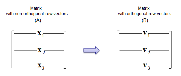
Figure 1. Orthogonalization of row vectors. The rows x₁, x₂, x₃ become mutually perpendicular rows v₁, v₂, v₃.

The picture below applies exactly the same idea to the columns. Nothing in the formulas changes. Only the way you read the vectors out of the matrix changes.

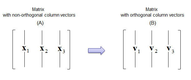
Figure 2. Orthogonalization of column vectors. The same process works on columns, which is the form used by the QR decomposition.

• The span is kept : v₁ to v_k span the same space as x₁ to x_k for every k. This is the property the result shares with the original matrix.
• The vectors themselves change : only v₁ equals its original. Every later vector loses its components along the earlier ones, so lengths and directions differ from the input.
• Orthogonal rows do not yet make an orthogonal matrix : in the strict sense, an orthogonal matrix Q has Q Q^T equal to the identity matrix, so its rows must also have length 1. The process gives perpendicular vectors, and a final normalization step gives unit length.
• A square determinant survives : each v_k is x_k minus a combination of earlier vectors, so V = L A with L lower triangular and ones on its diagonal. Therefore det(V) = det(A).

What are the steps of the process ?

Following is the process showing you derives the orthogonal matrix. If you just want to have algorithm, just copy this one as you need. But if you really want to understand the meaning of each step and how this process works, refer to Vector projection onto a Line first. Then these procedure would make more sense to you.

The formulas below handle three vectors. The first vector is taken as it is. Each later vector is the original minus one correction term for every vector already produced. So v₂ has one correction term, and v₃ has two. The pictures write a dot product with a centred dot. In the text of this page the vectors are rows, so the same dot product of x and v is written x v^T, as in the example later on.

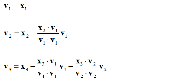
Figure 3. Gram Schmidt formulas for three vectors. Each new vector subtracts one correction term per vector already built.

The next formula is the general step for the n-th vector. It has n-1 correction terms, one for each of v₁ to v_n-1.

Figure 4. General Gram Schmidt step. The n-th vector subtracts its projection onto every earlier vector.

• Read x_n where the formula shows x₃ : Figure 4 starts with x₃ and uses x₃ in the first two numerators. The correct general step is v_n = x_n - (x_nv₁^T)/(v₁v₁^T) v₁ - ... - (x_nv_n-1^T)/(v_n-1v_n-1^T) v_n-1. The last term in the figure already has the correct x_n.
• The numerator always uses the original vector : x_nv_j^T takes the input vector x_n, while the denominator v_jv_j^T takes the new vector v_j.
• A zero vector means dependence : if some v_n comes out as the zero vector, x_n is a combination of the earlier inputs. Skip it, because the next step would divide by v_nv_n^T = 0.
• The order of the inputs matters : a different order gives a different set of perpendicular vectors. Only the first vector is kept unchanged.

What does each step mean ?

The formulas are easy to copy but hard to remember. They become easy to remember once each correction term is read as a projection, which is the length of one vector along the direction of another. The three pictures below take the formulas one line at a time.

If you look into the mathematical meaning of each step, it can be described as shown below.

Figure 5. The first step. The input x₁ is the reference direction and is copied to v₁ without change.

The second step, below, marks the correction term as the projection of x₂ onto v₁. Subtracting it leaves the part of x₂ that is perpendicular to v₁.

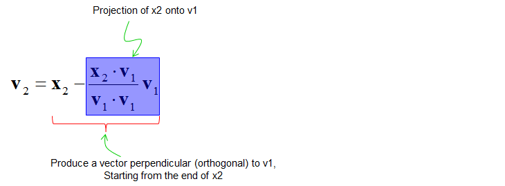
Figure 6. The second step. Removing the projection of x₂ onto v₁ leaves a vector perpendicular to v₁.

The third step, below, removes two projections, one onto v₁ and one onto v₂. The first bracket leaves a vector perpendicular to v₁, and the second bracket makes it perpendicular to v₂ as well.

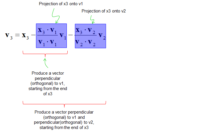
Figure 7. The third step. Removing both projections leaves a vector perpendicular to v₁ and to v₂.

• The subtraction is what creates the right angle : a vector minus its projection onto v_j has a zero dot product with v_j. You can check this by taking the dot product of both sides of the v₂ formula with v₁.
• One removal does not disturb another : v₁ and v₂ are already perpendicular. So removing the part along v₂ adds nothing back along v₁, and the two corrections can be done in either order.
• "Starting from the end of x" describes the drawing : the annotations picture the correction as an arrow drawn from the tip of x₂ or x₃. The result v_n itself is still a vector from the origin.

How is the process written with projections ?

Textbooks usually write the process with a projection operator, because it hides the fractions and shows the structure. The operator proj_u(x) = (xu^T)/(uu^T) u is the projection of x onto the line along u.

If you look into the concept of vector projection onto a line, you would easily understand that this process can be described as shown below.

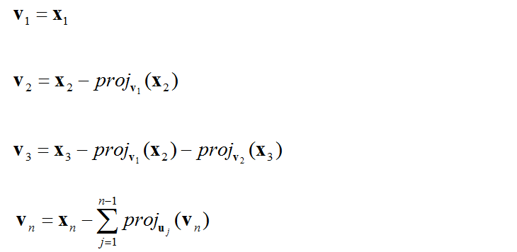
Figure 8. The process in projection form. Each new vector is its original minus the projections onto all earlier vectors.

• The v₃ line should project x₃ twice : Figure 8 writes proj_v1(x₂) in the v₃ line. The correct line is v₃ = x₃ - proj_v1(x₃) - proj_v2(x₃), which matches Figure 3.
• The general line should project x_n onto v_j : Figure 8 writes proj_uj(v_n) inside the sum. The correct form is v_n = x_n - Σ proj_vj(x_n), with j running from 1 to n-1. The vector being projected is the input x_n, and the direction is the new vector v_j.
• The sum is a projection onto a subspace : the terms together give the projection of x_n onto the space spanned by v₁ to v_n-1. So v_n is the part of x_n that the earlier vectors cannot represent.

Example

A small example with simple numbers is the best way to see every fraction appear. Watch the denominators in particular, because they come from the new vectors v_j and not from the inputs.

Let's assume that we are given a matrix as follows and assume that we want to orthogonalize the row vectors

Figure 9. The example matrix. Its determinant is 1, so the three rows are independent and the process gives three nonzero vectors.

At first, let's take out each row as vectors as follows.

Figure 10. The inputs x₁ = [1 -1 1], x₂ = [1 0 1] and x₃ = [1 1 2].

Now just plug in these vectors into each procedures and you will get the following result. (Note that the second vector in each inner product is transposed. This is to make inner product possible and produce a scalar value)

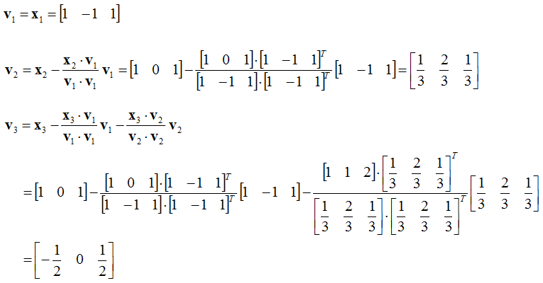
Figure 11. The worked calculation. The result is v₁ = [1 -1 1], v₂ = [1/3 2/3 1/3] and v₃ = [-1/2 0 1/2].

• v₂ needs one fraction : x₂v₁^T = 2 and v₁v₁^T = 3. So v₂ = [1 0 1] - (2/3)[1 -1 1] = [1/3 2/3 1/3].
• v₃ needs two fractions : x₃v₁^T = 2 over v₁v₁^T = 3 gives 2/3. Then x₃v₂^T = 5/3 over v₂v₂^T = 2/3 gives 5/2. So v₃ = [1 1 2] - (2/3)[1 -1 1] - (5/2)[1/3 2/3 1/3] = [-1/2 0 1/2].
• The second line of the v₃ expansion should start from x₃ : Figure 11 writes [1 0 1], which is x₂, as the first vector and in the first numerator. Both should be x₃ = [1 1 2]. The final answer [-1/2 0 1/2] is correct, and it is what the correct substitution gives.

How can you be sure that the result is orthogonal ?

A hand calculation needs its own check, because one wrong fraction makes every later vector wrong. The error also stays hidden, since the wrong result still looks like a plausible set of vectors.

Now we have completed the calculation. Then you may ask how we can be sure that the answer is correct ?

One way to prove it is to draw the resulting vectors into a coordinate and check if the angles between each vector are 90 degree.

The plots below draw the inputs on the left and the results on the right, all starting from the origin. On the right, v₁ is the longest vector, and v₂ and v₃ are much shorter, because their lengths are √(2/3) and √(1/2).

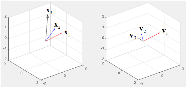
Figure 12. Input vectors on the left and orthogonalized vectors on the right. A 3D view makes the right angles hard to judge by eye.

However this kind of graphical method can be an easy and quick method in 2 vectors (2 Dimensional), but in 3 vectors, it is difficult to measure the angles between vectors correctly. If it goes more than 3, it is impossible to apply this kind of graphical method.

More accurate way is to take the innerproduct of all the two combination from the resulting matrix. In case of this example, take the following inner product. If you get '0' for all of these, it means that you derived a correct orthogonal matrix.

Figure 13. The three pairwise inner products to check. All three are 0 for this example.

• v₁v₂^T = 0 : 1/3 - 2/3 + 1/3 = 0.
• v₁v₃^T = 0 : -1/2 + 0 + 1/2 = 0.
• v₂v₃^T = 0 : -1/6 + 0 + 1/6 = 0.
• One matrix product does all the checks at once : with V holding v₁, v₂, v₃ as rows, V V^T must be diagonal. Here it is diag(3, 2/3, 1/2). The diagonal holds the squared lengths, and every off-diagonal entry is an inner product that must be 0.
• A computer result is zero only up to rounding : in floating point, expect values such as 1e-16 rather than exact zeros. Compare against a small tolerance.

How do you get an orthonormal matrix and the QR decomposition ?

Most applications need unit vectors as well as right angles. So the usual last step divides each v_k by its length. The resulting set is orthonormal, and the matrix that holds it is an orthogonal matrix in the strict sense.

For the example, the lengths are √3, √(2/3) and √(1/2). The normalized rows are therefore q₁ = [1 -1 1]/√3, q₂ = [1 2 1]/√6 and q₃ = [-1 0 1]/√2. With these rows in Q, Q Q^T = I holds exactly.

Keeping the fractions you computed along the way gives more than Q. Write the inputs as columns of A^T. Then A^T = Q^T R, where R is upper triangular. For this example, the rows of R are [√3 2/√3 2/√3], [0 √(2/3) 5/√6] and [0 0 1/√2]. This is the QR decomposition, and Gram Schmidt is the most direct way to compute it by hand.

• R records the projections : each entry above the diagonal of R is x_nq_j^T, the length of an input along an earlier unit vector. Each diagonal entry is the length of v_n.
• Library QR may flip signs : numpy.linalg.qr on the same columns returns the same q vectors up to sign. For this matrix it negates q₁ and q₂ and the matching rows of R. Both answers are valid.
• Classical Gram Schmidt loses accuracy on nearly dependent vectors : rounding errors pile up, and the computed vectors drift away from perpendicular. Modified Gram Schmidt, which removes each projection from the running vector, or a Householder QR is the usual choice in numerical code.
• The determinant check still works : det(A) = 1 here, and the product of the three lengths √3 x √(2/3) x √(1/2) is also 1.