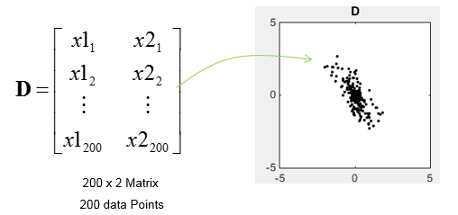
In this application, I will use SVD to find the principal components for a data set. Principal components means the axis (a vector) that represents the direction along which the data is most widely distributed, i.e the axis with the largest variance. In this example, I will use a 200 x 2 matrix which represents the 200 data points as plotted below.

This page takes one step further than the PCA page. Once SVD has found the principal axes, the same factors can project every data point onto one axis. We only set one singular value to zero and multiply the factors back together. The result is the orthogonal projection of the data onto the principal axis and onto the minor axis.

• What is the data set and its SVD ?
• How does zeroing one singular value project the data ?
• Matlab code for the projection

What is the data set and its SVD ?

Let's first fix the data and its SVD, because the projection is built from nothing else. The data set is the same one as on the PCA page. So the axes and the singular values below are the same numbers that page found.

First I assinged the D matrix to Matrix M. There is no mathmatical reason to do this. I just did this because I wanted to use the matrix M for all the matlab examples for this page.

Then I did SVD as follows.

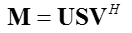
For this D, the SVD gives σ₁ = 14.6873 and σ₂ = 4.9745. The first row of transpose(V) is v₁ = (-0.4940, 0.8695), the principal axis, and the second row is v₂ = (0.8695, 0.4940), the minor axis. U is 200 x 200 and S is 200 x 2, with the two singular values on its diagonal and zeros everywhere else.

• D has rank 2 : it has two nonzero singular values, so its rows fill the whole plane. A projection onto one axis reduces the rank to 1.
• The squares of the singular values split the data : σ₁² + σ₂² = 215.72 + 24.75 = 240.46 is the sum of the squared lengths of all 200 points. The principal axis holds 89.7 % of it.
• v₁ and v₂ are unit vectors at a right angle : so each data point splits uniquely into a part along v₁ and a part along v₂. The projection keeps one of the two parts.

How does zeroing one singular value project the data ?

Now we come to the actual projection. The idea is to keep one term of the SVD and drop the other. Setting σ₂ to zero keeps only the part of D along the principal axis, and setting σ₁ to zero keeps only the part along the minor axis.

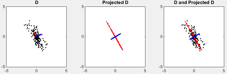
D in the following plots represents the data set in scatter plot. You would intuitively find an axis along which the data are spread most widely. tr(V) shows two row vectors in transpose(V) vector that came from SVD. You see the red arrow is pointing the princial components, i.e the major axis. The third plot shows the transpose(V) vectors overlayed onto the data set. (Matlab  source code for this example is in < List 1 >)

The plots in the table below are not the same as on the PCA page, although the sentence above repeats its wording. The first plot shows D with the two axes of tr(V). The middle plot shows the projected points, red for DrMajor on the principal axis and blue for DrMinor on the minor axis. The third plot overlays both projections on D.

In the table, the red 0 marks the singular value that was set to zero. Smajor keeps σ₁ and Sminor keeps σ₂. Multiplying each one back with U and V^T gives two new 200 x 2 matrices, as the equations below show.

D       = U S VT      = σ1 u1 v1T + σ2 u2 v2T

DrMajor = U Smajor VT = σ1 u1 v1T = D v1 v1T
DrMinor = U Sminor VT = σ2 u2 v2T = D v2 v2T

DrMajor + DrMinor = D

v1 v1T = [ 0.2440 -0.4295 ; -0.4295  0.7560 ]
v2 v2T = [ 0.7560  0.4295 ;  0.4295  0.2440 ]      sum = identity

Why is the first term a projection? If you multiply D = U S V^T on the right by v₁, you get D v₁ = σ₁ u₁. So σ₁ u₁ v₁^T = D v₁ v₁^T. For one data point d, which is one row of D, this row becomes (d . v₁) v₁^T. That is the length of d along the unit vector v₁, times v₁, which is exactly the orthogonal projection of d onto the principal axis. The matrix v₁ v₁^T is the projection matrix, and applying it twice changes nothing.

• The red points lie on one line : DrMajor has rank 1, so every red point sits on the principal axis. The same holds for the blue points on the minor axis.
• Each point is the sum of its two projections : DrMajor + DrMinor = D, because the two projection matrices add up to the identity matrix. The red and the blue part of a point are at a right angle.
• The error of the projection is σ₂ : the distance from D to DrMajor, in the Frobenius norm, is σ₂ = 4.9745. So the red points keep 89.7 % of the squared length of the data, and the blue points hold the other 10.3 %.
• No other line does better : by the Eckart-Young theorem, the principal axis gives the smallest total squared distance of any line through the origin. That is why this projection is the basis of dimensionality reduction.

Matlab code for the projection

The listing below produced the plots above. It generates the same data as the PCA page, takes the SVD, and then builds Smajor and Sminor by copying S and setting one diagonal entry to zero.

< List 1 >

clear all;

N = 200;
rng(1);
t = rand(1,N);
rng(1);
r = randn(1,N);
x1 = 0.5 .* r .* cos(2*pi*t);
x2 =1.5 .* r .* sin(2*pi*t);

M = [x1; x2];
tm = [cos(pi/6) -sin(pi/6);sin(pi/6) cos(pi/6)]
D = (tm * M)';
x = D(:,1);
y = D(:,2);
M = D;

[U,S,V]=svd(M);

vT = V';
vT1 = vT(1,:);
vT2 = vT(2,:);

sigma1 = S(1,1);
sigma2 = S(2,2);

Smajor = S;
Smajor(2,2) = 0;
Sminor = S;
Sminor(1,1) = 0;

DrMajor = U * Smajor * V';
DrMinor = U * Sminor * V';

subplot(1,3,1);
plot(x,y,'ko','MarkerFaceColor',[0 0 0],'MarkerSize',2);
axis([-5 5 -5 5]);
hold on;
quiver(0,0,vT1(1),vT1(2),'r','MaxHeadSize',1.5,'linewidth',2);
axis([-5 5 -5 5]);
hold on;
quiver(0,0,vT2(1),vT2(2),'b','MaxHeadSize',1.5,'linewidth',2);
axis([-5 5 -5 5]);
hold off;
title('D');

subplot(1,3,2);
plot(DrMajor(:,1),DrMajor(:,2),'ro','MarkerFaceColor',[1 0 0],'MarkerSize',2);
axis([-5 5 -5 5]);
hold on;
plot(DrMinor(:,1),DrMinor(:,2),'bo','MarkerFaceColor',[0 0 1],'MarkerSize',2);
axis([-5 5 -5 5]);
title('Projected D');
hold off;

subplot(1,3,3);
plot(x,y,'ko','MarkerFaceColor',[0 0 0],'MarkerSize',2);
axis([-5 5 -5 5]);
hold on;
plot(DrMajor(:,1),DrMajor(:,2),'ro','MarkerFaceColor',[1 0 0],'MarkerSize',2);
axis([-5 5 -5 5]);
hold on;
plot(DrMinor(:,1),DrMinor(:,2),'bo','MarkerFaceColor',[0 0 1],'MarkerSize',2);
axis([-5 5 -5 5]);
title('Projected D');
hold off;
title('D and Projected D');;

A few details are useful if you reuse this listing. The full SVD returns U as a 200 x 200 matrix, but only its first two columns reach the result, so svd(M,'econ') gives the same DrMajor and DrMinor with less memory. The first subplot is titled 'D', but it also draws the two axis arrows from tr(V). In the third subplot, the title is set twice, and only the last one, 'D and Projected D', appears. The listing also calls rng(1) before both rand and randn, so t and r come from the same random sequence.