A Taylor series rebuilds a function near one point from the function's own derivatives at that point. The result is a polynomial, which is easy to evaluate, differentiate and integrate. On this page I'll go through what the series looks like and why it is useful. Then I'll show where the formula comes from and how far from the point it can be trusted. The exponential and the sine function serve as the worked examples.

• What does a Taylor series look like ?
• Why is a Taylor series useful ?
• What is a Maclaurin series ?
• Example 1 : Taylor and Maclaurin Series of Exponential Function
• Where does the Taylor formula come from ?
• How far from the point a can you trust the series ?

What does a Taylor series look like ?

Tayler Series is a kind of technique to approximate any form of smooth function around a specific point in the form of polynimial function. Let's look at the following illustration as an example. Let's suppose that we are given a function called f(x) that is plot in green curve. Now look at the graph plotted in red. As you see, the red plot has exactly same value as f(x) at the point 'a' and within a certain range (marked as orange background) the red graph is almost same as the green graph (f(x)). In this case, we can say the red plot is a approximation of green plot (f(x)) around the point 'a'.

Then you may ask 'how can we get (derive) the equation for the red graph ?'. One of th enswer to this question is Taylor Series as described below.

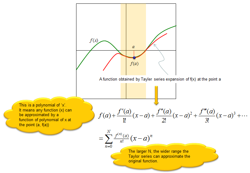
Figure 1. A Taylor series matches f(x) at the point a, and its polynomial follows f(x) closely in a range around that point.

• Green curve : the original function f(x).
• Red curve : the polynomial from the Taylor series at the point a. It touches f(x) at (a, f(a)) and stays close to it inside the orange band. Outside the band the two curves separate.
• The formula : each term uses one derivative of f at the point a, divided by n!, and multiplied by (x - a)ⁿ. The sum up to N is the polynomial of degree N.
• The left cloud : says that any function can be approximated. This needs a smooth function, one with as many derivatives at a as the polynomial has terms. A function with a corner at a, such as |x| at 0, has no Taylor series there.
• The right cloud : says that a larger N gives a wider range. This holds only inside the radius of convergence of the series. The last section of this page shows a case where extra terms make the result worse.

Why is a Taylor series useful ?

Now you would ask 'Why we need or use this kind of series expression ?'. Before I answer to this question, let me ask a question to you first. When do we use 'approximation' ? Approximation is just 'similar value' but not exact/accurate value. So it cannot be as good as the exact value. Then why do we still use approximation sometimes ?

It is because it is easy to use or easy to calculate even though we need to sacrifice a certain degree of accuracy.

This logic applies to Taylor Series as well. Taylor series is a approximation to a given function which may have similarity to the original function only within a certain range. But we still use this series because it is easy to use and simple to calculate in many case.

You may think 'look at the series equation.. it doesn't look simple.. it has a lot of derivatives (it may scare you) and equations gets very long.

Many people tend to think 'An equation is very complicated or hard if it is very long', but it is not true. 'Length of a equation' and level of difficulty is completely different story. Even though the Taylor expanded equation tend to be long, all the derivative terms (f'(a), f''(a), f'''(a)) will become a constant if you plug in a specific 'a' value. So the expanded equation (the series) become a polynomial of the variable 'x'. The polynomial function is one of the most common function everybody learned in high school math. However long it is, we don't feel much difficulties understanding/solving the equation.

So the main usage of Taylor series is to approximate a function with a simple polynomial function which is well known to everybody.

Engineers use the first one or two terms all the time, often without calling them a Taylor series. The first-order series f(a) + f'(a)(x - a) is the tangent line at a. Replacing a nonlinear system by this line near its operating point is called linearization, and most control and circuit analysis starts there. Three common cases are listed below.

• sin x ≈ x for a small angle : at x = 0.1 rad the error is 0.17 %, and at x = 0.5 rad it is 4.3 %. The error comes mainly from the next term, x³/6.
• e^x ≈ 1 + x for a small x : e^0.1 = 1.10517, and the approximation gives 1.1.
• √(1 + x) ≈ 1 + x/2 for a small x : √1.1 = 1.04881, and the approximation gives 1.05.

• A Taylor series trades accuracy for simplicity : the polynomial is easy to handle, and the error is small near a.
• The first-order series is the tangent line : this is the basis of linearization.
• The first dropped term sets the error : for sin x ≈ x, the error is close to x³/6.

What is a Maclaurin series ?

Similar to Taylor series, there is another special series called Maclaurin Series. Actually Maclaurin Series is just a special form of Taylor Series. Taylor Series is an approximation of a function at any point 'a', but Maclaurin Sieries is an approximation at the point '0'. It means if you replace 'a' in Taylor serious with '0', you will get Maclaurin Series equation.

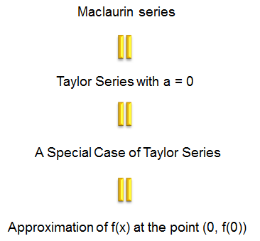
Figure 2. A Maclaurin series is a Taylor series with a = 0, so it approximates f(x) near the point (0, f(0)).

Because a = 0, every term is a plain power of x, f⁽ⁿ⁾(0) xⁿ / n!. The table below lists the Maclaurin series that appear most often in engineering. The last column gives the range of x for which the infinite series equals the function.

• A Maclaurin series is a Taylor series at a = 0 : every result for Taylor series applies to it.
• Choose a close to the x you need : a Maclaurin series is convenient, but it is not the best choice when x is far from 0. Example 1 shows the difference in numbers.

Example 1 : Taylor and Maclaurin Series of Exponential Function

In this example, we are given an exponential function. Can we approximate this function in the form of polynomial ? The exponential is the easiest function to start with, because every derivative of e^x is e^x itself. So every coefficient of the series comes from the single value e^a.

Yes, we can get the approximation using Taylor series expansion as follows. And if you plug '0' into 'a' in the derived Taylor series equation, you will get the Maclaurin series for the exponential function.

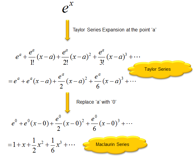
Figure 3. Taylor series of e^x at a, and the Maclaurin series that follows from a = 0.

• Taylor series : every derivative at a is e^a, so the terms are e^a(x - a)ⁿ/n!. The second line only evaluates 2! = 2 and 3! = 6.
• Maclaurin series : with a = 0, e⁰ = 1, and the series becomes 1 + x + x²/2 + x³/6 + ...

Let's check how fast the Maclaurin series approaches the true value. The table below adds the terms one by one for x = 0.5 and for x = 2. The column N gives the highest power that is included.

For x = 0.5, six terms give six correct digits. For x = 2, even nine terms are still off in the third digit, because x is far from a = 0. Moving a closer helps a lot. To compute e^2.1, take the Taylor series at a = 2 with three terms, e²(1 + 0.1 + 0.005) = 8.1649. The exact value is 8.1662. The Maclaurin series with the same three terms gives 1 + 2.1 + 2.205 = 5.305, which is useless.

• Every coefficient of e^x is e^a/n! : the exponential is its own derivative.
• The error shrinks fastest near a : for the same number of terms, x = 0.5 is far more accurate than x = 2.
• Pick the expansion point near x : three terms at a = 2 give e^2.1 to four digits, and three terms at a = 0 do not.

Where does the Taylor formula come from ?

The formula looks as if it came from nowhere, but it follows from one simple demand. We want a polynomial p(x) that behaves like f(x) at the point a. So we ask that p and f have the same value at a, the same slope, the same second derivative, and so on.

Write the polynomial in powers of (x - a), p(x) = c₀ + c₁(x - a) + c₂(x - a)² + c₃(x - a)³ + ... At x = a every term except c₀ is 0, so p(a) = c₀. Differentiate once and set x = a, and only c₁ is left. Differentiate twice, and only 2c₂ is left. In general, the n-th derivative at a is n! c_n, because the power (x - a)ⁿ gives n(n-1)...1 = n! after n derivatives.

Setting each of these equal to the matching derivative of f gives the coefficients directly.

c_n = f⁽ⁿ⁾(a) / n!

That is exactly the formula in Figure 1. The n! in the denominator is not a convention. It cancels the n! that the n-th derivative of (x - a)ⁿ produces.

When the series stops at the power N, the difference between f and the polynomial is the remainder. In the Lagrange form, R_N(x) = f^(N+1)(ξ) (x - a)^N+1 / (N+1)!, where ξ is some point between a and x. For e^0.5 with N = 3, the largest possible value of the derivative is e^0.5. So the error is at most e^0.5 x 0.5⁴/24 = 0.0043. The actual error in the table above is 0.0029, inside that bound.

• The coefficients come from matching derivatives : p and f agree in value and in the first N derivatives at a.
• The n! cancels the derivatives of the power : the n-th derivative of (x - a)ⁿ is n!.
• The remainder gives an error bound : it grows with the distance |x - a| and shrinks with the factorial (N+1)!.

How far from the point a can you trust the series ?

The pictures so far show the polynomial following the function only near a. So the natural question is whether more terms push that range out forever. For some functions they do. For others there is a hard limit, called the radius of convergence, and beyond it the series fails no matter how many terms you add.

Let's look at a function where more terms do help. The Maclaurin series of sin x converges for every x. The plot below draws sin x together with its Maclaurin polynomials of degree 1, 3, 5 and 7, from -2π to 2π.

Figure 4. sin x and its Maclaurin polynomials. Each higher degree follows the sine further away from 0, but every polynomial leaves the sine at some distance.

• Degree 1 : the line y = x, which is the small-angle approximation. It is good only close to 0.
• Degree 3 : x - x³/6 stays close up to about x = 1 and then falls away. It crosses 0 at x = √6 = 2.45, where the sine is still positive.
• Degree 5 and 7 : each follows the sine further out. The degree 7 polynomial stays close up to about x = π.
• Far from 0 : every polynomial goes to plus or minus infinity, while sin x stays between -1 and 1.

At x = 3 the partial sums are 3, -1.5, 0.525, 0.0911, 0.1453, 0.1409 and 0.1411, and sin 3 = 0.1411. Seven terms are needed here, while at x = 1 three terms already give 0.8417 against 0.8415. So the series works everywhere, but the price grows with the distance from a.

Now take 1/(1 - x), whose Maclaurin series is 1 + x + x² + ... This series converges only for |x| < 1. At x = 2 the function equals -1, but the partial sums are 1, 3, 7, 15, 31, ..., and they grow without limit. The limit comes from the point x = 1, where the function itself goes to infinity. The series of ln(1 + x) has the same radius, and at x = 1 it converges only slowly. Eight terms give 0.6345 against ln 2 = 0.6931.

One more warning completes the picture. The function e^-1/x2, set to 0 at x = 0, is smooth, and all of its derivatives at 0 are 0. So its Maclaurin series is 0 for every x, even though the function is not 0 anywhere except at x = 0. Smoothness is necessary for a Taylor series, but it does not guarantee that the series equals the function.

• More terms help only inside the radius of convergence : for 1/(1 - x) at a = 0 that radius is 1, and outside it the partial sums diverge.
• Series of e^x, sin x and cos x converge for every x : but far from a they need many terms.
• A singularity limits the radius : the series of 1/(1 - x) cannot reach past the point x = 1, where the function goes to infinity.
• Check the error, not only the formula : the remainder term or a numerical comparison tells you whether N terms are enough.