A WCDMA downlink constellation on a signal analyzer rarely looks like the clean QPSK you expect. The reason is that the Node B sends many code channels at once, and the analyzer shows their sum. Let's follow the signal chain in 25.213 first, then look at a measured example, and finally build the pattern by hand from two QPSK channels.

• How does the Node B build one downlink signal ?
• What does a measured downlink constellation look like ?
• How do two QPSK channels create the pattern ?
• Reference

How does the Node B build one downlink signal ?

To understand the constellation, we first need to know where in the chain the channels are added together. 25.213 splits the downlink transmitter into three steps, and each step has its own figure.

If you combine the following three sections in 25.213, you will have a overall downlink physical channel flow as shown below.

• 5.1 Spreading (Figure 8)
• 5.1.5 Channel combining (Figure 9)
• 5.3.2 Modulation (Figure 11)

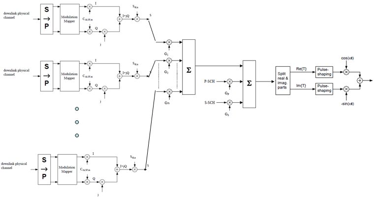
Figure 1. Downlink transmitter chain from 25.213. Every physical channel is spread and scrambled on its own, and then all channels are added into one complex chip stream before modulation.

• On the left, each downlink physical channel passes a serial to parallel converter and a modulation mapper. The mapper splits the symbols into an I branch and a Q branch.
• Both branches are multiplied by the same channelisation code C_ch,SF,m. The Q branch is then multiplied by j and added to the I branch, which gives I+jQ.
• The complex chips are multiplied by the downlink scrambling code S_dl,n. The output is point S of 25.213 Figure 8.
• In the middle, each channel is weighted by its own gain G₁ to G_n and summed. P-SCH and S-SCH are added with their own gains G_P and G_S, without spreading or scrambling.
• On the right, the sum is split into real and imaginary parts, pulse shaped, and modulated onto cos and -sin carriers.

The important point for the constellation is the order of these steps. Each channel is a clean QPSK signal at its own point S. But the Node B never transmits one channel alone. It transmits the weighted sum, and the sum is what the receiver sees at chip level.

• Spreading does not change the QPSK shape : the channelisation code is real-valued, so it only flips the sign of both I and Q together.
• Scrambling rotates the points : a complex scrambling chip moves each QPSK point, and all channels under one scrambling code move together.
• The gains G_i decide the pattern : channels with different power produce the rings and clusters seen on the analyzer.

What does a measured downlink constellation look like ?

Now let's compare the theory with a real measurement. The example below is a Release 99 downlink, where every channel for data transfer uses QPSK. The result still does not look like QPSK, and this section explains why.

Assuming the all the physical channel for data transfer is using QPSK (Release 99), the constellation is shown as below. (Graph on left shows Code Domain Power for each channel and the right side graph shows the constellation).

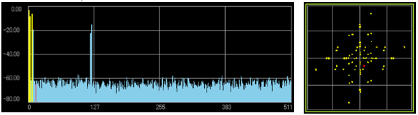
Figure 2. Measured code domain power and composite constellation. A few active code channels with different power give a scattered, many point constellation.

• The left plot is code domain power. The horizontal axis runs from code 0 to 511, and the vertical axis runs from 0 to -80 dB.
• A few strong bars stand at the lowest code numbers, and one more bar stands near code 120. Everything else is at the noise floor of about -60 dB.
• The right plot is the constellation of the same signal. It shows many points spread around the centre, not four QPSK points.

When I first saw this constellation, I was very confused because it is so much different from my expectation of QPSK constellation.

This kind of complicated constallation comes from the vector summation of multiple QPSK with different amplitudes. If only one channel is transmitted, you would have a normal QPSK constellation as you expected, but if multiple channel (multiple QPSK) are summed, you would get various different patters depending on how many channels are summed and what is the amplitude of each QPSK channel.

There are two different constellations that an analyzer can show, and it helps to keep them apart. The composite constellation shows the descrambled chips of the whole signal, so it contains the sum of all channels. The code domain constellation shows the symbols of one channel after despreading with its own channelisation code. Despreading removes the other channels, because the OVSF codes are orthogonal. So the same signal shows a clean QPSK in the code domain view, and a crowded pattern in the composite view.

The number of active channels also changes the picture. With two channels, the pattern is regular and easy to explain, as the next section shows. With several channels at different power, the points overlap and the plot looks almost random, which is the case in Figure 2.

• A composite constellation is a chip-level sum : it shows all code channels at once, so it is not a modulation quality view of any single channel.
• Check one channel in the code domain : despreading with the channel's own code gives the QPSK that the channel really carries.
• More channels give a denser pattern : the plot depends on how many channels are on and on their relative power.

How do two QPSK channels create the pattern ?

The measured plot has too many channels to follow point by point. So let's reduce the problem to two QPSK channels and change only their amplitude ratio. Then each point in the result can be traced back to one pair of input symbols.

Assuming there is just two QPSK channels are being transmitted, I created two example cases with two different amplitude combination as follows.

The plots below show the two cases side by side. In each case, the rows show channel x1, then channel x2, and then the two together. The left column of each case is ideal, and the right column adds noise.

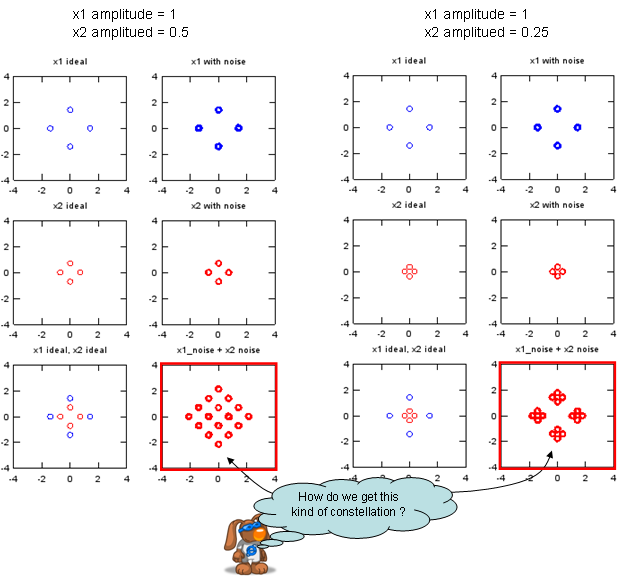
Figure 3. Sum of two QPSK channels. With an amplitude ratio of 0.5, the sum gives 16 separate points. With a ratio of 0.25, the sum gives four tight clusters of four points.

• In the left case, x1 has amplitude 1 and x2 has amplitude 0.5. In the right case, x2 has amplitude 0.25.
• Each QPSK channel is drawn with its four points on the I and Q axes. The x1 points sit at about 1.4 from the centre.
• The bottom left plot of each case overlays the two ideal channels. The bottom right plot, marked in red, is the sum with noise.
• With the 0.5 ratio, the 16 sums form a diamond of separate points. With the 0.25 ratio, each x1 point gets a small cluster of four points around it.

The count is easy to check. Channel x1 has 4 possible symbols and channel x2 has 4 possible symbols, so the sum x1 + x2 has 4 x 4 = 16 possible values. When x2 is small, the 16 values stay close to the 4 points of x1, so they look like 4 clusters. When x2 grows toward x1, the clusters spread and merge into one diamond of 16 points. With three channels, the count becomes 4 x 4 x 4 = 64, and the plot fills up quickly.

The axis orientation has a reason as well. A QPSK chip of the form +/-1 +/- j, multiplied by a scrambling chip of the same form, always lands on the I axis or the Q axis. For example, (1+j)(1+j) = 2j and (1+j)(1-j) = 2. So after scrambling, each QPSK channel shows four points on the axes, which is the orientation in these plots.

Following sequence of graph show you how each of the constellation spot at the final result can created from two original QPSK constellation.

Each small panel pair below picks one symbol of x1 in blue and one symbol of x2 in red. The panel to its right marks, in black, the point that their sum produces in the 16 point diamond.

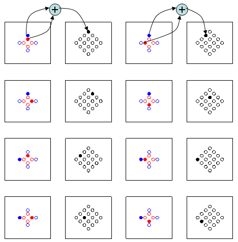
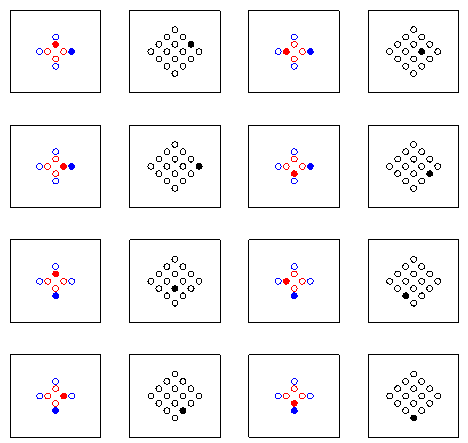
Figure 4. Symbol pairs and their sums. Each of the 16 combinations of one x1 symbol and one x2 symbol lands on a different point of the diamond.

• The plus sign at the top of the upper plot shows the operation: the blue x1 point and the red x2 point are added.
• Within one row, x1 stays the same and x2 changes. So one x1 symbol produces a group of four neighbouring sums.
• Across both plots there are 16 panels with a black point, one for each pair, and no two pairs share a point.

• N QPSK channels give up to 4^N points : two channels give 16 points and three give 64, if their amplitudes differ enough.
• The amplitude ratio sets the shape : a small second channel gives clusters, and a larger one gives a spread diamond.
• The pattern is not a modulation error : a crowded composite constellation is normal for a WCDMA downlink.

Reference

• 3GPP TS 25.213 v19.0.0 - subclause 5.1 Spreading and Figure 8, 5.1.5 Channel combining and Figure 9, 5.3.2 Modulation and Figure 11