A polynomial is the first function you meet whose graph is neither a straight line nor a single parabola. It can turn several times, cross the x-axis at several points, and head up or down at each end. Let's go through the tools you need to handle it. The first is the generic form and the degree. The next two are the graph and Descartes rule of signs, which tells you how many roots to look for. Then comes the symmetry test for even and odd functions. The last is polynomial division, which is how you actually find the roots.
- What is Polynomial Function ?
- How to Graph ?
- Descartes rule of signs
- Even and odd functions
- Polynomial Division
What is Polynomial Function ?
Polynomial Function is an expression of more than two algebraic terms, especially the sum of several terms that contain different powers of the same variable(s). it can be express in a generic form as shown below.

Let's name the parts of that expression, because the rest of the page uses them. Each piece such as bxn-1 is a term, and the number in front of x is its coefficient. The highest power n is the degree, and its coefficient a is the leading coefficient. The last term d has no x, so it is called the constant term.
The powers of x must be whole numbers, 0 or larger. So 3x2 + x-1 and 2√x are not polynomials, because their powers are -1 and 1/2. The definition above says more than two terms, but in algebra the word is wider than that. A single term such as 5x3 and a two-term expression such as x - 2 are polynomials too. Some coefficients can also be zero. For example, x4 - 3x2 + 1 is a degree 4 polynomial with no x3 term and no x term.
The degree is the first thing to read, because it limits what the graph can do. A polynomial of degree n has at most n real roots. Its graph also has at most n - 1 turning points, where it changes from going up to going down.
The degree is the highest power of x : It limits the number of real roots to n and the number of turning points to n - 1.The degree and the leading coefficient fix the end behaviour : The next section uses only these two numbers to decide where the graph starts and ends.Every power must be a whole number : A negative or fractional power of x gives a different kind of function, not a polynomial.
How to Graph ?
You can graph any polynomial functions by both hands(harder method) and technology(easier method). Technology gives an exact picture, but a hand sketch shows you why the graph has its shape. So let's focus on the hand method, which needs only three pieces of information.
When graphing with hands, you need to know the x-intercepts(also known as roots), y-intercept, and end behaviours of the function. Some of the tips you can use for drawing by hands are
- When a polynomial function is in its standard form, you must factor the equation in order to find the roots
- You can use both synthetic division and long division to factor the function
- If a polynomial function is an even degree function with positive sign, the end behaviour is quadrant 2 to quadrant 1. However if the function has a negative sign, the end behaviour is quadrant 3 to quadrant 4
- If a polynomial function is an odd degree function with positive sign, the end behaviour is quadrant 3 to quadrant 1. However if the function has a negative sign, the end behaviour is quadrant 2 to quadrant 4
- End behaviours are ALWAYS from left to right
< Quadrant on a Cartesian Coordinate >
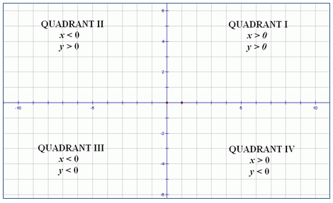
The sign in those tips is the sign of the leading coefficient. The reason is that the highest power grows faster than all the other terms together. So for a large |x|, the leading term alone decides whether f(x) is a large positive or a large negative number.
Let's put the tips together on one example, f(x) = x3 - 2x2 - 5x + 6. The Polynomial Division section below shows how to factor it into (x - 1)(x + 2)(x - 3). So the roots are x = 1, x = -2 and x = 3. The y-intercept is f(0) = 6, which is simply the constant term. The degree is 3 and the leading coefficient is +1, so the end behaviour is quadrant 3 to quadrant 1.
The graph below plots this function. The red points are the three roots, and the green point is the y-intercept. Between two neighbouring roots the graph does not change sign, so it makes one hump or one dip there.
Figure 1. Graph of f(x) = (x - 1)(x + 2)(x - 3). The three roots, the y-intercept and the end behaviour are enough to sketch the whole shape of this cubic.
The sign between roots comes from one test point : f(0) = 6 is positive, so the graph is above the axis between -2 and 1. Next, f(2) = -4 is negative, so it is below the axis between 1 and 3.A cubic turns at most twice : This one turns near x = -0.79, at a height of about 8.2, and near x = 2.12, at a height of about -4.06. A hand sketch does not need these exact values.A repeated root touches the axis instead of crossing it : With a factor (x - 1)2, the graph reaches the axis at x = 1 and turns back. A factor repeated three times crosses the axis but flattens as it crosses.
Descartes rule of signs
This rule is used to identify the number of positive roots, negative roots, and/or imaginary Roots of a polynomial function. By the application of this rule, you can identify whether you found the correct roots or not.
- If a polynomial function of f(x) has n sign changes, there are n positive roots, or fewer than n by an even number such as n - 2 or n - 4
- If f(-x) has m sign changes, there are m negative roots, or fewer than m by an even number
- Degree of function = total Number of positive and Negative root(s) and number of imaginary root(s), when a repeated root is counted as many times as it repeats and x = 0 is not a root
Why fewer by an even number? A polynomial with real coefficients has its imaginary roots in pairs, a + bi and a - bi. So the number of real roots can only drop two at a time. When you count sign changes, skip any term whose coefficient is 0. If x = 0 is a root, factor out x first and apply the rule to what is left.
Let's apply the rule to g(x) = x4 + 3x3 + x2 - 2x - 5, the same polynomial as the Synthetic Division example below. Its signs are + + + - -. They change once, from +x2 to -2x, so g has exactly one positive root. Next, g(-x) = x4 - 3x3 + x2 + 2x - 5. Its signs are + - + + -, which change three times. So g has 3 or 1 negative roots.
The degree is 4, so only two cases are possible. In the first, g has 1 positive root, 3 negative roots and no imaginary roots. In the second, g has 1 positive root, 1 negative root and 2 imaginary roots. A numerical solver gives the real roots x = 1.131 and x = -2.604 and the imaginary pair -0.764 +/- 1.055i. So the second case is the real one.
The sign changes give an upper limit : The actual count equals that limit or drops from it in steps of two, because imaginary roots come in pairs.f(-x) counts the negative roots : Replacing x with -x flips the sign of every odd power. The positive roots of f(-x) are the negative roots of f(x).The rule is a check, not a solver : It tells you how many roots to look for, and it never tells you where they are.
Even and odd functions
Symmetry is another shortcut for graphing, after the roots and the end behaviour. If a function is even or odd, you only need to draw half of its graph. The test uses f(-x), the same substitution as Descartes rule of signs.
Odd function is a function with a point symmetry, proved by f(-x)=-f(x), x can be any real numbers
Even function is a function with a line symmetry, proved by f(x) = f(-x), x can be any real numbers
Point symmetry here means symmetry about the origin, and line symmetry means symmetry about the y-axis. So an even function looks the same when you mirror it in the y-axis. An odd function looks the same after a half turn around the origin. This saves work when you graph, because you can draw the right half and copy it to the left.
For a polynomial the test is quick. A polynomial is odd when every power of x is odd, such as x3 - x. It is even when every power is even, such as x4 - 3x2 + 1, and the constant term counts as the power x0. The degree alone does not decide it. For example, x3 + 1 has an odd degree, but f(-x) = -x3 + 1. That is neither f(x) nor -f(x), so x3 + 1 is neither even nor odd.
Most polynomials are like that. The graphing example x3 - 2x2 - 5x + 6 mixes odd and even powers, so Figure 1 has no symmetry about the y-axis or the origin.
Even means symmetric about the y-axis : f(-x) = f(x), and a polynomial with only even powers passes this test.Odd means symmetric about the origin : f(-x) = -f(x), and a polynomial with only odd powers passes this test.An odd degree does not make a function odd : Check every power, not only the highest one. A polynomial that mixes both kinds of power is neither even nor odd.
Polynomial Division
Division is the step that turns a polynomial in standard form into factors, and the factors give the roots. The divisor is usually a linear factor such as x - 2. The result is written as divisor x quotient + remainder. The example below writes it as P(x)Q(x)+R(x), where P(x) is the divisor, Q(x) the quotient and R(x) the remainder.
Synthetic Division
Synthetic division is a shortcut for dividing by a linear factor x - c. It works only with the coefficients, so a missing power must be written with a coefficient of 0. The example divides a degree 4 polynomial by x - 2, so c = 2 is the number on the left of the table.

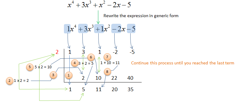
Write the answer in P(x)Q(x)+R(x) format
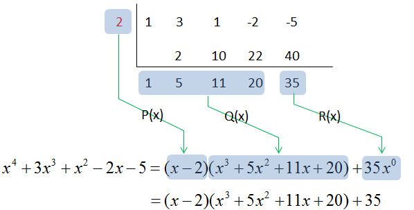
Let's read the table in the two diagrams above. Bring down the first coefficient 1. Multiply it by 2 and write the product 2 under the next coefficient 3. Add them to get 5, and repeat the multiply and add until the last column. The bottom row 1, 5, 11, 20 gives the quotient x3 + 5x2 + 11x + 20, one degree lower than the original. The last number 35 is the remainder.
You can check the result by expanding it. The product (x - 2)(x3 + 5x2 + 11x + 20) is x4 + 3x3 + x2 - 2x - 40, and adding 35 gives back the constant term -5. For a divisor ax - b with a different from 1, divide by x - b/a first and then divide the quotient by a.
Remainder and Factor Theorem
The remainder 35 above is not a coincidence. The Remainder Theorem says that dividing f(x) by x - c leaves the remainder f(c). Here f(2) = 16 + 24 + 4 - 4 - 5 = 35, which matches the last number in the table.
The Factor Theorem follows directly. If f(c) = 0, the remainder is 0, so x - c is a factor of f(x). This is how the graphing example was factored. When the leading coefficient is 1, every integer root divides the constant term. So for f(x) = x3 - 2x2 - 5x + 6 you try +/-1, +/-2, +/-3 and +/-6.
The first try already works, because f(1) = 1 - 2 - 5 + 6 = 0. Synthetic division by x - 1 then gives the bottom row 1, -1, -6 with a remainder of 0. So the quotient is x2 - x - 6, which factors as (x - 3)(x + 2). The full result is f(x) = (x - 1)(x + 2)(x - 3).
Synthetic division needs a linear divisor : It divides by x - c. For a divisor of degree 2 or higher, use long division.The remainder equals f(c) : Evaluating f(c) is a quick check on the last number of the table.A zero remainder means a factor : Each factor x - c you find gives a root c and a quotient one degree lower, so you repeat until a quadratic is left.