|
Mechanical Engineering |
||
|
Coriolis Motion
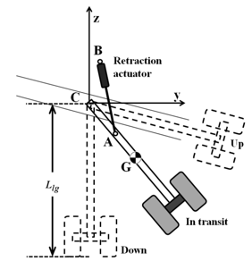
Coriolis motion refers to simultaneous translational and rotational motion of an object. The motion of hydraulic cylinders for construction equipment and aircraft landing gears are practical examples of Coriolis motion, where the piston exhibits a translational motion along the rotating cylinder. Pressurized hydraulic fluid is used to drive the piston. Following shows an example of a Coriolis motion in a landing gear actuator. The end Point (point A) of the Rectraction Actuator is the part undergoing Coriolis Motion.
Image Source : “An Integrated Approach to Vehicle, Propulsion System, and Subsystem Sizing - Application to the All Electric Aircraft ([1])
Let point A be the point of reference and point B be the object that experiences a Coriolis motion. For all Coriolis motion problems, there are the fixed XYZ and rotating xyz coordinate systems. Then the Coriolis velocity (eq. 1) and acceleration (eq.2) at point B are expressed as follows:
where,
Example 01 >
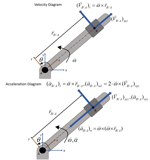
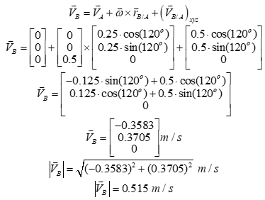
Collar B slides away from point A along the rotating rod at 0.5 m/s with an acceleration of 0.1 m/s2. The rod rotates about point A, where point A is fixed by a pin joint. Additionally, the rod rotates at 0.5 rad/s with an acceleration of 0.05 rad/s2 in the counter-clockwise direction. Calculate the Coriolis velocity and acceleration of Collar B at the instant where and the overall distance between points A and B is 0.25 m. The velocity and acceleration diagrams are shown below.
where X,Y represents the fixed coordinate system and x,y represents the moving coordinate system.
Example 02 > Matlab Excercise
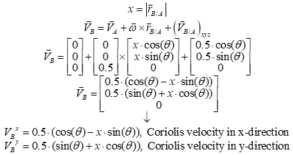
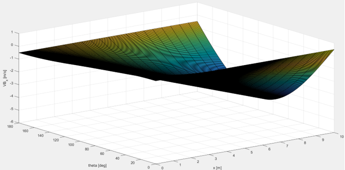
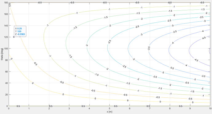
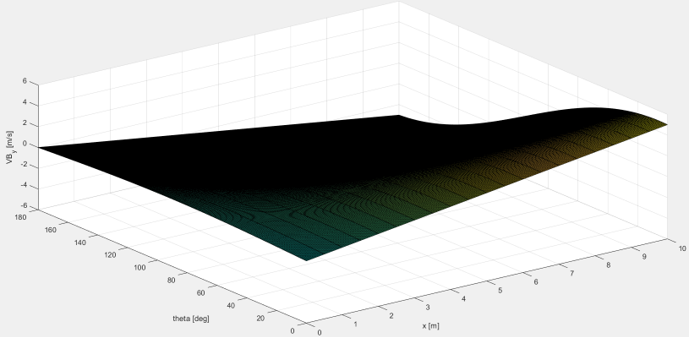
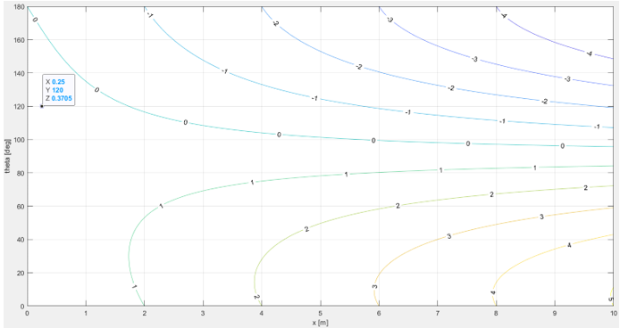
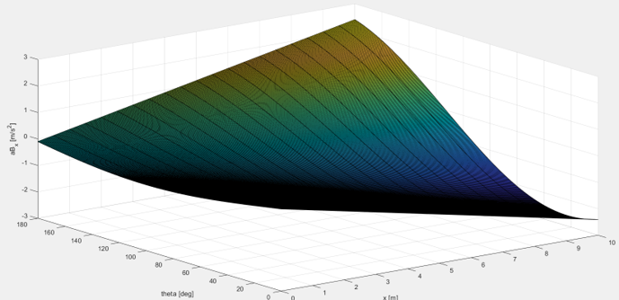
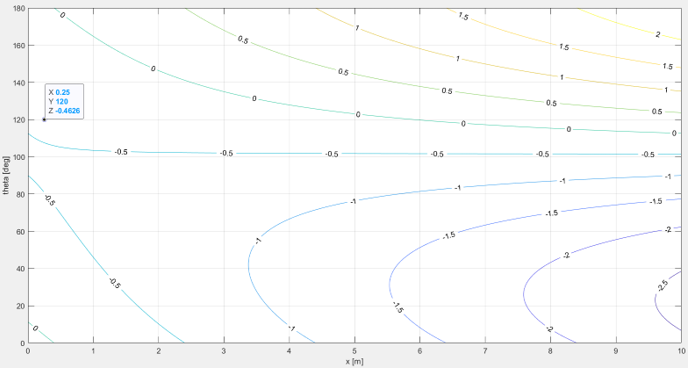
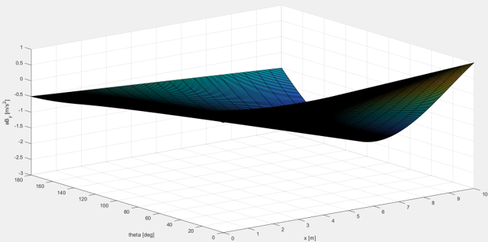
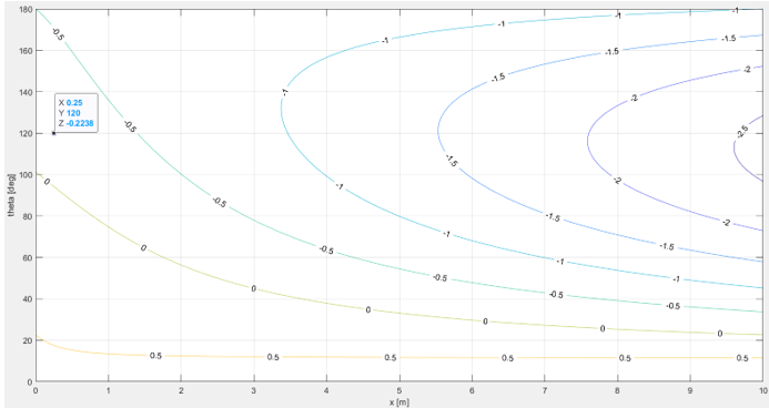
Using MATLAB, create the contour and surface plots that represent the Coriolis velocity and acceleration of collar B in x and y directions from example 1 with respect to the rod orientation and the overall distance between the points A and B. All the velocities and accelerations are identical to example 1. The rod orientation ranges from 0 to 180 degrees and the overall distance ranges from 0 to 10 meters. The contour plots should also indicate the final answers from example 1. There should be 4 sets of contour and surface plots in total.
Step 1: Derive the symbolic expressions for the Coriolis velocity and acceleration components.
Step 2: MATLAB Implementation.
% Example 2 % Define the lower and upper bounds of x and theta x_range = [0,10]; theta_range = [0,180];
% Define the Coriolis velocity and acceleration as functions. VB_x=@(theta,x) 0.5*(cosd(theta)-x.*sind(theta)); VB_y=@(theta,x) 0.5*(sind(theta)+x.*cosd(theta));
% Create the surface and contour plots. [x,theta] = meshgrid(x_range(1,1):0.5:x_range(1,2),theta_range(1,1):0.5:theta_range(1,2)); figure(1) surf(x,theta,VB_x(theta,x)) xlabel('x [m]'); ylabel('theta [deg]'); zlabel('VB_x [m/s]'); grid on
figure(2) contour(x,theta,VB_x(theta,x),'ShowText','on') hold on; plot3(0.25,120,VB_x(120,0.25),'bo') hold off; xlabel('x [m]'); ylabel('theta [deg]'); grid on
figure(3) surf(x,theta,VB_y(theta,x)) xlabel('x [m]'); ylabel('theta [deg]'); zlabel('VB_y [m/s]'); grid on
figure(4) contour(x,theta,VB_y(theta,x),'ShowText','on') hold on; plot3(0.25,120,VB_y(120,0.25),'bo') hold off; xlabel('x [m]'); ylabel('theta [deg]'); grid on
figure(5) surf(x,theta,aB_x(theta,x)) xlabel('x [m]'); ylabel('theta [deg]'); zlabel('aB_x [m/s^2]'); grid on
figure(6) contour(x,theta,aB_x(theta,x),'ShowText','on') hold on; plot3(0.25,120,aB_x(120,0.25),'bo') hold off; xlabel('x [m]'); ylabel('theta [deg]'); grid on
figure(7) surf(x,theta,aB_y(theta,x)) xlabel('x [m]'); ylabel('theta [deg]'); zlabel('aB_y [m/s^2]'); grid on
figure(8) contour(x,theta,aB_y(theta,x),'ShowText','on') hold on; plot3(0.25,120,aB_y(120,0.25),'bo') hold off; xlabel('x [m]'); ylabel('theta [deg]'); grid on
MATLAB Outputs
< Coriolis velocity in x-direction >
< Coriolis velocity in y-direction >
< Coriolis acceleration in x-direction >
< Coriolis acceleration in y-direction >
Example 03 > Matlab Excercise
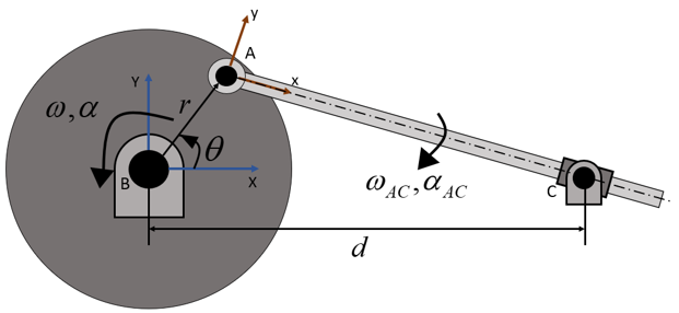
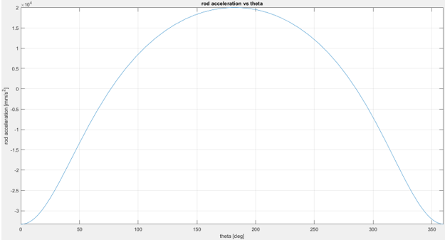
Derive the mathematical models of the angular velocity, angular acceleration, translational velocity, and translational acceleration of the rotating rod depicted in figure 10 using MATLAB. The translational velocity and acceleration corresponds to the velocity and acceleration of the rod sliding along the collar, respectively. The collar rotates about point C, where such a point is fixed by a pin joint. Additionally, create the following plots with 0 <≤ θ <≤ 360, r = 250 mm, d = 1000 mm, ω = 10 rad/s, and α = 2 rad/s:
Following is the diagram describing the problem.
MATLAB Code
% Example 3 syms theta omega alpha r d syms omega_AC alpha_AC syms v_stroke a_stroke
% Inputs % alpha : Angular acceleration of the wheel [rad/s^2] % d : Distance between the pin joints. % omega : Angular velocity of the wheel [rad/s] % r : Wheel radius [mm] % theta : Input angle to the wheel [deg]
% Outputs % omega_AC : Angular velocity of the rod [rad/s] % v_stroke : Translational velocity of the rod along the rotating collar % [mm/s] % alpha_AC : Angular acceleration of the rod [rad/s^2] % a_stroke : Translational acceleration of the rod along the rotating % collar [mm/s^2]
% Compute the symbolic expression for the translational and angular % velocities of the rod.
% Derive the equations for the translational velocity at point C. vA = cross([0;0;omega],[r*cosd(theta);r*sind(theta);0]); v_stroke_x = v_stroke*(r*cosd(theta) - d)/((r*cosd(theta) - d)^2 + (r*sind(theta))^2)^0.5; v_stroke_y = v_stroke*(r*sind(theta))/((r*cosd(theta) - d)^2 + (r*sind(theta))^2)^0.5; C = vA + cross([0;0;-omega_AC],[d-r*cosd(theta);-r*sind(theta);0]) + [v_stroke_x;v_stroke_y;0]; % Must assume clockwise rotation for omega_AC.
% Create the A and B matrices for Ax = B using the translational velocity % equations at point C, implying that the translational velocity at point C is % equal to zero as point C is fixed. x = [omega_AC;v_stroke]. [A,B] = equationsToMatrix([vC(1,1),vC(2,1)],[omega_AC,v_stroke]);
% Compute the expressions for the angular and translational velocities of % the rod using the A and B matrices. X_vel = simplify(linsolve(A,B));
% Derive the equations for the translational velocity at point C. aA = cross([0;0;alpha],[r*cosd(theta);r*sind(theta);0]) - omega^2*[r*cosd(theta);r*sind(theta);0]; aC_A_t = cross([0;0;-alpha_AC],[d-r*cosd(theta);-r*sind(theta);0]); aC_A_n = cross([0;0;-omega_AC],cross([0;0;-omega_AC],[d-r*cosd(theta);-r*sind(theta);0])); % Must assume clockwise rotation for omega_AC.
aC_A_t_stroke = cross([0;0;-2*omega_AC],[v_stroke_x;v_stroke_y;0]); % Must assume clockwise rotation for omega_AC. a_stroke_x = a_stroke*(r*cosd(theta) - d)/((r*cosd(theta) - d)^2 + (r*sind(theta))^2)^0.5; a_stroke_y = a_stroke*(r*sind(theta))/((r*cosd(theta) - d)^2 + (r*sind(theta))^2)^0.5; aC = aA + aC_A_t + aC_A_n + aC_A_t_stroke + [a_stroke_x;a_stroke_y;0];
% Create the A and B matrices for Ax = B using the translational % acceleration equations at point C, implying that the translational acceleration % at point C is equal to zero as point C is fixed. x = [alpha_AC,a_stroke]. [A,B] = equationsToMatrix([aC(1,1),aC(2,1)],[alpha_AC,a_stroke]);
% Compute the expressions for the angular and translational accelerations of % the rod using the A and B matrices. X_accel = simplify(linsolve(A,B));
% Define the anonymous functions that represent the rod velocities and % accelerations. Note that this step must be done after executing all the % codes above.
% Define the input parameters. omega = 10; alpha = 2; d = 1000; r = 250;
% omega_AC(theta) corresponds to X_vel(1,1) and v_stroke corresponds to X_vel(2,1). omega_AC=@(theta) -(omega*r*(r - d*cos((pi*theta)/180)))/(d^2 - 2*cos((theta*pi)/180)*d*r + r^2); v_stroke=@(theta) -(d*omega*r*sin((pi*theta)/180))/(d^2 + r^2 - 2*d*r*cos((theta*pi)/180))^(1/2);
% alpha_AC(theta) corresponds to X_accel(1,1) and a_stroke corresponds to X_accel(2,1). % Ensure that both of the functions above are used for the functions below. alpha_AC=@(theta) (2*d^2*omega_AC(theta)*v_stroke(theta) + 2*omega_AC(theta)*r^2*v_stroke(theta) - alpha*r^2*(d^2 - 2*cos((theta*pi)/180)*d*r + r^2)^(1/2) + alpha*d*r*cos((pi*theta)/180)*(d^2 - 2*cos((theta*pi)/180)*d*r + r^2)^(1/2) - 4*d*omega_AC(theta)*r*v_stroke(theta)*cos((pi*theta)/180) - d*omega^2*r*sin((pi*theta)/180)*(d^2 - 2*cos((theta*pi)/180)*d*r + r^2)^(1/2))/(d^2 + r^2 - 2*d*r*cos((theta*pi)/180))^(3/2); a_stroke=@(theta) -(d^2*omega_AC(theta)^2 + cos((theta*pi)/180)*d*omega^2*r - 2*cos((theta*pi)/180)*d*omega_AC(theta)^2*r + alpha*sin((theta*pi)/180)*d*r - omega^2*r^2 + omega_AC(theta)^2*r^2)/(d^2 + r^2 - 2*d*r*cos((theta*pi)/180))^(1/2);
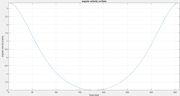
% Create the plots that show the relationship between the input angle and % rod velocities and accelerations. figure (1) fplot(omega_AC,[0 360]) xlabel('theta [deg]'); ylabel('angular velocity [rad/s]'); title('angular velocity vs theta'); grid on;
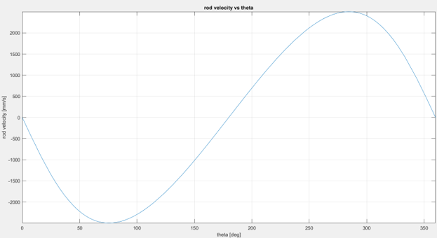
figure (2) fplot(v_stroke,[0 360]) xlabel('theta [deg]'); ylabel('rod velocity [mm/s]'); title('rod velocity vs theta'); grid on;
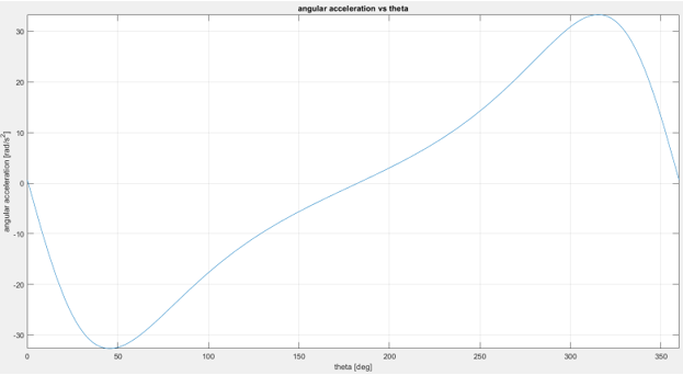
figure (3) fplot(alpha_AC,[0 360]) xlabel('theta [deg]'); ylabel('angular acceleration [rad/s^2]'); title('angular acceleration vs theta'); grid on; figure (4) fplot(a_stroke,[0 360]) xlabel('theta [deg]'); ylabel('stroke acceleration [mm/s^2]'); title('stroke acceleration vs theta'); grid on;
< Relationship between the input angle and angular velocity of the rod >
< Relationship between input angle and translational velocity of the rod >
< Relationship between input angle and angular acceleration of the rod >
< Relationship between input angle and translational acceleration of the rod >
Reference :
[1] I. Chakraborty et al., “An Integrated Approach to Vehicle, Propulsion System, and Subsystem Sizing - Application to the All Electric Aircraft, ” Proceedings of the Institution of Mechanical Engineers Part G Journal of Aerospace Engineering, June 2015. doi: 10.1177/0954410015594399.
|
||
