Mechanical Engineering

Inverse Kinematics

Inverse kinematics is a mathematical problem solving method used to solve for the actuator inputs using the known position of an end effector, in which is a device that is used to interact with its surrounding environment. Such a problem solving method is commonly used to design robotic arms for various industry applications, where the robotic gripper (or any other device that is attached to the end of a robotic arm) is the end effector. Inverse kinematics is used to calculate the orientation of robotic arms using the known end effector position.

Figure 1 depicts an example of a robotic arm with the end effector labelled, where the end effector interacts with a cardboard box in a warehouse setting.

< Figure 1: Robotic arm in a warehouse setting  >

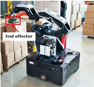
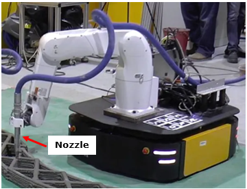
Figure 2 depicts an example of a robotic arm that is used for 3D printing, where the nozzle is the end effector.

< Figure 2: 3D printing with a robotic arm  >

Unlike inverse kinematics, forward kinematics is used to evaluate the kinematic joint positions and kinematic linkage orientations of multi-body dynamic systems using known actuator inputs (i.e., initial and final orientations of the linkage driven by an actuator). Forward kinematics is taught in second and third year dynamics courses for mechanical and aerospace engineering students. Introduction to Robotics is an example of a fourth-year mechanical and aerospace engineering elective that teaches inverse kinematics for design and analysis of robotic mechanisms. The equations of motion for both forward and inverse kinematics are no different. However, inverse kinematics is harder than forward kinematics because often times there are either no feasible solutions, there are multiple possible solutions, or there is a feasible solution. For forward kinematics, one can analytically find a feasible solution for the final linkage orientations and joint positions using trigonometry analysis.

Inverse kinematics of a dual-arm robot

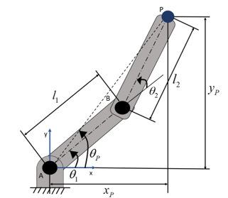
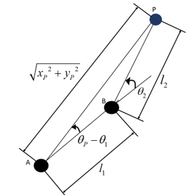
Figure 3 depicts the configuration of a dual-arm robot with a known position of the end effector (indicated as point P) in both x and y directions relative to the fixed pin-joint, as well as linkage lengths without out-of-plane motion. Inverse kinematics is used to evaluate the linkage orientations. As such a robot is a simple mechanism, a closed-form analytical solution can be used to solve the problem.

< Figure 3: Configuration of the dual-arm robot. Joint B is a kinematic joint. >

Step 1: Outline the equations of motion for the end effector.

where

Step 2: Illustrate the triangle formed by joints A, B, and P (shown in figure 4).

< Figure 4: Triangle formed by the joints and the end effector.>

Step 3: Derive the expression for link AB orientation using the cosine law for the triangle from step 2.

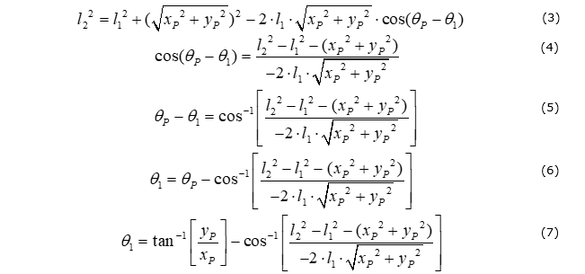
As all the variables for equation 7 are known, the equation can be used to calculate the orientation of link AB relative to the global x-axis.

Step 4: Derive the expression for link BP orientation (measured relative to the orientation of link AB) using one of the equations of motion.

If the other equation of motion was used instead, then:

Example 1: Inverse kinematics of a dual-arm robot with MATLAB

The trajectory of the end effector of a dual-arm robot with l1 = 0.5 m and l2 = 0.5 m is represented by the following equation:

First, determine the value of xp and yp (i.e., f(xp)) at which the robot arms are fully extended, using the fzero function for MATLAB. xp,max and yp,max represent the end effector position in x and y directions when the robot arms are fully extended, respectively. Print the final solution with 3 decimal places.

MATLAB Code

% Inputs

% L1 : Length of the lower arm [m]

% L2 : Length of the upper arm [m]

% xP : Position of the end effector in x-direction [m]

% yP : Position of the end effector in y-direction

% Outputs

% xP_max : Position of the end effector in x-direction at which the arms

% are fully extended [m].

% yP_max : Position of the end effector in y-direction at which the arms

% are fully extended [m].

% theta_1 : Orientation of the lower arm with respect to the global x-axis

% [deg].

% theta_2 : Orientation of the upper arm with respect to the lower arm

% [deg].

% Define the constants.

L1 = 0.5; L2 = 0.5;

% Define the function that represents the trajectory of the end effector.

f=@(xP) -0.75*xP^2 + 0.995;

% Compute the value of xP_max using the fzero function.

% When the arms are fully extended,

% (L1 + L2)^2 = (xP^2 + (f(xP))^2)^2

% Create the anonymous function for the root solving problem.

F=@(xP) (xP^2 + (f(xP))^2) - (L1 + L2)^2;

% Compute xP_max and yP_max. The solution should exist in between x = 0 and x = L1 + L2.

xP_max = fzero(F, [0 L1+L2]);

yP_max = f(xP_max); % Back-substitute xP_max into the trajectory equation.

% Output the solution.

fprintf('The position of the end effector is xP = %1.3f m, yP = %1.3f m when the arms are fully extended. \n', xP_max, yP_max)

MATLAB Output

The position of the end effector is xP = 0.946 m, yP = 0.323 m when the arms are fully extended.

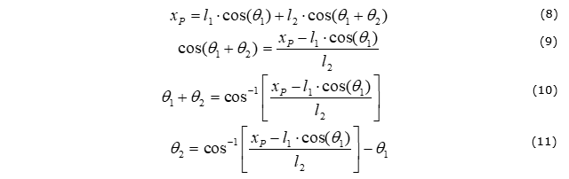
Then create plots to show the robot arm orientations from x = 0 to x = xP,max using MATLAB. Use equations 7 and 11 for the lower and upper arm orientations, respectively. Both of the plots should be created in the same space.

MATLAB Code

% Plot the robot arm orientations.

% Define the functions that represent the robot arm orientations.

theta_1=@(xP) atand(f(xP)/xP) - acosd((L2^2 - L1^2 - xP^2 - (f(xP))^2)/(-2*L1*(xP^2 + (f(xP))^2)^0.5));

theta_2=@(xP) acosd((xP - L1*cosd(theta_1(xP)))/L2) - theta_1(xP);

figure(1)

theta_1_plot = fplot(theta_1,[0 xP_max], 'r-');

hold on

theta_2_plot = fplot(theta_2,[0 xP_max], 'b-');

xlabel('xP [m]'); ylabel('theta [deg]');

title('theta vs xP');

legend([theta_1_plot, theta_2_plot],{'lower arm orientation (theta_1)', 'upper arm orientation (theta_2)'})

grid on;

MATLAB Output

< Figure 5: Orientation of the robot arms with respect to the position of the end effector in the x-direction. >

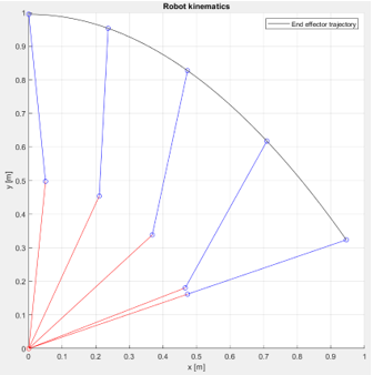
Finally, create wireframe models to show 5 different robot arm configurations from x = 0 to x = xP,max, as well as the plot of the end effector trajectory from x = 0 to x = xP,max. All the plots should be in the same space to show the motion of the entire robot arm.

MATLAB Code

% Plot the end effector trajectory and the robot arm configurations.

% Create the arrays of x and y values for joints A, B, and the end effector P.

xP = linspace(0,xP_max,5);

N = numel(xP); % Number of elements in the xP array.

yP = zeros(1,N); xB = zeros(1,N); yB = zeros(1,N);

for i = 1:N

    xB(1,i) = L1*cosd(theta_1(xP(1,i)));

    yB(1,i) = L1*sind(theta_1(xP(1,i)));

    yP(1,i) = yB(1,i) + L2*sind(theta_1(xP(1,i)) + theta_2(xP(1,i)));

end

xA = zeros(1,N); yA = zeros(1,N);

% Create the plots that shows the robot arm motion.

figure(2)

hold on; grid on;

xlabel('x [m]'); ylabel('y [m]');

title('Robot kinematics');

x_plot_1 = zeros(N,2); y_plot_1 = zeros(N,2);

x_plot_2 = zeros(N,2); y_plot_2 = zeros(N,2);

for i = 1:N

    x_plot_1(i,1) = xA(1,i); x_plot_1(i,2) = xB(1,i);

    y_plot_1(i,1) = yA(1,i); y_plot_1(i,2) = yB(1,i);

    x_plot_2(i,1) = xB(1,i); x_plot_2(i,2) = xP(1,i);

    y_plot_2(i,1) = yB(1,i); y_plot_2(i,2) = yP(1,i);

    % Plot the kinematic joints and connect the joints using lines.

    arms = plot(x_plot_1(i,:),y_plot_1(i,:),'ro-',x_plot_2(i,:),y_plot_2(i,:),'bo-');

    % Plot the end effector trajectory.

    traj = fplot(f,[0 xP_max],'k-');

    legend(traj,'End effector trajectory')

    daspect([1 1 1]); % Square grids for all the plots in the loop

end

< Figure 6: Wireframe model of the dual-arm robot motion. The red line represents the lower arm and the blue line represents the upper arm. >

Reference :

[1]