Recurrent Neural Networks (RNNs) are a class of neural networks designed for processing sequential data by maintaining a form of memory across time steps. Unlike traditional feedforward networks that treat each input independently, RNNs are structured to capture temporal dependencies by passing information from one step of the sequence to the next through hidden states. This makes them particularly effective for tasks where context and order are essential, such as language modeling, speech recognition, and time-series forecasting. The recurrent connections within the network allow it to learn patterns that span multiple time steps, enabling it to make predictions based on both current inputs and previously seen data.

It is designed to process sequential data by maintaining a hidden state that captures information from previous inputs, making them particularly suited for tasks like natural language processing, speech recognition, and time-series analysis. Unlike traditional feedforward neural networks, RNNs incorporate loops that allow them to reuse computations across sequences, effectively modeling temporal dependencies and context.

Why RNN ?

Recurrent Neural Networks (RNNs) are used because they are uniquely suited to handle sequential data where the order and context of elements matter. Traditional neural networks lack the capability to retain information from previous inputs, making them ineffective for tasks like language translation, speech recognition, or time-series prediction. RNNs address this limitation by incorporating loops within the network that allow information to persist across time steps, enabling the model to learn from the sequence and dependencies within the data. This ability to model temporal dynamics and maintain context over time is what makes RNNs a powerful tool for problems where understanding the sequence as a whole is crucial.

• RNNs are designed to handle sequential or time-dependent data effectively.
• They maintain a hidden state that captures information from previous time steps, enabling memory of past inputs.
• Ideal for tasks where context and order are important, such as:
• Language modeling
• Machine translation
• Speech recognition
• Time-series forecasting
• Unlike feedforward networks, RNNs can process inputs of varying lengths.
• They learn temporal dependencies, making them useful for predicting future events based on past observations.
• Enable modeling of dynamic behaviors in data over time.
• Can be trained to generate output sequences, making them suitable for text generation or music composition.
• Serve as the foundation for more advanced models like LSTMs and GRUs, which address RNN limitations like vanishing gradients.

What were there before RNN ?

RNN is desgined mainly to forecast (predict) something mostly along the axis of time (i.e, temporal axis). What kind of techniques were used for this before RNN ?

We can think of this in the context of conventional statistical method and in the context of neural network.

In the context of convenstional statistical method, time-series forecasting and sequence modeling were primarily handled using traditional statistical methods and linear models. Techniques such as Autoregressive (AR), Moving Average (MA), Autoregressive Integrated Moving Average (ARIMA), and Exponential Smoothing were commonly used to predict future values based on past observations. These models were grounded in statistical theory and often relied on assumptions of linearity and stationarity, which limited their ability to capture complex, non-linear patterns in data. While effective for certain types of structured and well-behaved data, these approaches struggled with tasks requiring the modeling of long-term dependencies or contextual relationships, which later made RNNs a more powerful alternative in many forecasting applications.

Speaking of neural networ, before the advent of RNNs, most neural network-based models for prediction and classification relied on feedforward neural networks. These networks process inputs in a single pass—from input to output—without any mechanism to retain or refer back to previous inputs. Common architectures included Multilayer Perceptrons (MLPs), which were widely used for tasks like classification, regression, and simple pattern recognition. While MLPs could approximate complex functions, they lacked the ability to model sequences or temporal dependencies because they treated each input independently.To handle sequential data, early attempts with MLPs often involved manually engineering features—such as including lagged variables or using fixed-size sliding windows over time-series data. However, these approaches were limited in flexibility and scalability, especially when the temporal relationships were long or variable in length. The introduction of RNNs marked a significant breakthrough by embedding memory and recurrence directly into the architecture, enabling neural networks to naturally process sequences and learn from them over time, something feedforward networks couldn't do effectively.

Conventional Statistical Methods

• Common Techniques:
  • Autoregressive (AR)
  • Moving Average (MA)
  • Autoregressive Integrated Moving Average (ARIMA)
  • Exponential Smoothing
• Strengths:
  • Grounded in statistical theory
  • Effective for short-term prediction with well-behaved data
  • Useful for structured and stationary datasets
• Limitations:
  • Assumes linearity and stationarity
  • Incapable of capturing complex, non-linear dependencies
  • Poor at modeling long-term relationships or context

Neural Network-Based Approaches (Before RNNs)

• Common Techniques:
  • Feedforward Neural Networks (Multilayer Perceptrons - MLPs)
  • Manual feature engineering with lagged variables
  • Fixed-size sliding windows to simulate time dependence
• Strengths:
  • Capable of modeling complex, non-linear functions
  • Effective for classification and regression tasks
• Limitations:
  • Each input is treated independently
  • No memory or state retention across time steps
  • Manual preprocessing makes scaling to longer sequences difficult

What RNN Introduced

• Built-in memory through hidden states and loops
• Ability to learn from temporal dependencies naturally
• More powerful for sequence tasks like text, audio, and time-series data

Challenges/Limitations

Despite their strengths in handling sequential data, Recurrent Neural Networks (RNNs) come with several inherent challenges and limitations that can affect their performance and scalability. One of the most well-known issues is the problem of vanishing and exploding gradients, which arises during backpropagation through time and hampers the network’s ability to learn long-term dependencies. RNNs also tend to be computationally expensive due to their sequential nature, making parallelization difficult and training slower compared to feedforward networks. Additionally, they can struggle with retaining information over long sequences and are sensitive to input length and initial conditions. These limitations have led to the development of more advanced architectures like Long Short-Term Memory (LSTM) and Gated Recurrent Units (GRU), which were specifically designed to address some of the shortcomings of traditional RNNs.

• Vanishing Gradient Problem
  • Gradients shrink exponentially during backpropagation through time (BPTT).
  • Prevents effective learning of long-range dependencies.
  • Training slows down or stalls completely.
• Exploding Gradient Problem
  • Gradients grow excessively during training, causing instability.
  • Leads to large weight updates and erratic learning behavior.
  • Often requires techniques like gradient clipping to stabilize.
• Difficulty Learning Long-Term Dependencies
  • Standard RNNs struggle to retain information over long sequences.
  • They tend to forget earlier inputs due to limited memory capacity.
• Sequential Computation Bottleneck
  • Processes inputs one step at a time, making parallelization difficult.
  • Leads to slower training compared to feedforward architectures.
• Sensitivity to Input Length and Initialization
  • Performance can degrade with highly variable sequence lengths.
  • Heavily influenced by initial weights and hidden state values.
• Exposure Bias During Training
  • During training, the model uses ground-truth outputs from previous steps.
  • During inference, it relies on its own predictions, leading to error accumulation.
• Limited Representational Power
  • Lacks built-in mechanisms like gates to control information flow.
  • Less flexible compared to LSTM or GRU networks.
• Prone to Overfitting on Small Datasets
  • High model complexity makes them overfit when data is limited.
  • Regularization techniques like dropout are harder to apply effectively in recurrent layers.

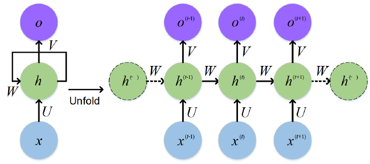
Architecture

The architecture of a RNN is designed to process sequences of data by incorporating loops that allow information to persist across time steps. At its core, an RNN consists of an input layer, a hidden layer with recurrent connections, and an output layer. Unlike feedforward networks, where data flows in a single direction, RNNs maintain a hidden state that is updated at each time step based on both the current input and the previous hidden state. This recursive structure enables the network to retain memory of previous inputs and to use this contextual information when processing the current input. The same set of weights is shared across all time steps, making the model efficient and consistent for sequential data processing. This unique architectural design allows RNNs to model temporal patterns and dependencies, which are essential for tasks like language modeling, speech recognition, and time-series prediction.

The most common representation of RNN architecture is illustrated as below. The left side shows the compact version of a single RNN cell, and the right side shows the network unfolded in time. At each time step t, the RNN receives an input x(t), updates its hidden state h(t) based on the current input and the previous hidden state h(t−1), and produces an output o(t). This process allows the model to maintain a temporal memory, capturing dependencies across time steps. All time steps share the same weight matrices U, W, and V, enabling consistent transformation across the sequence.

Source : Audio visual speech recognition with multimodal recurrent neural networks

Followings are breakdown of this diagram and short descriptions on each component.

• Input x(t): Represents a single element in a sequence.
  • Example: In a sentence, x(t−1) = "The", x(t) = "weather", x(t+1) = "is"
• Hidden state h(t): Encodes information from previous time steps.
  • Captures context such as "The weather" at time step t
• Output o(t): Produced from the hidden state.
  • In text generation, o(t) might be "is"
  • In speech recognition, it could be a phoneme or word probability
• Weight matrices:
  • U: Transforms input x(t) to hidden state space
  • W: Transmits hidden state from h(t−1) to h(t)
  • V: Maps hidden state h(t) to output o(t)
• Temporal Recurrence:
  • Each RNN cell passes context forward using h(t), allowing the model to learn sequence dependencies

NOTE : Details on input and outputs at each step (Example of Word Prediction Task)

Assuming the RNN is used for a next-word prediction task based on the input sequence:

• x(t−1) = "The"
• x(t) = "weather"
• x(t+1) = "is"

Output o(t−1) (After input "The")

Predicted next word distribution:

• "weather": 0.6
• "sun": 0.2
• "sky": 0.1
• "man": 0.1

Most likely prediction: "weather"

Output o(t) (After input "weather")

Predicted next word distribution:

• "is": 0.7
• "was": 0.2
• "feels": 0.1

Most likely prediction: "is"

Output o(t+1) (After input "is")

Predicted next word distribution:

• "nice": 0.5
• "cold": 0.3
• "bad": 0.2

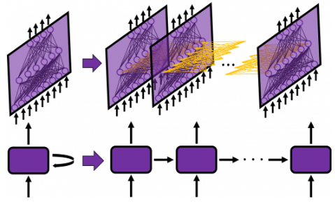
Most likely prediction: "nice"

Each output o(t) is typically a probability distribution over the vocabulary, and the word with the highest score can be selected as the prediction.

Following is another example of RNN architecture. I think this is a better representation for time-series prediction. In this context, the RNN processes a sequence of numerical inputs arriving over time—such as stock prices, temperatures, or sensor readings—and generates future predictions based on patterns it has learned. The top portion of the image shows the unfolding of network layers across time, while the bottom abstractly represents this behavior through a chain of RNN cells that pass hidden states forward. This enables the model to retain memory of past data and make context-aware predictions for future points in the series.

Source : Simple RNN: the first foothold for understanding LSTM

Followings are breakdown of the illustration and description for each component

• Top Layer (Neural Layer Over Time):
  • Each slanted panel represents a neural network operating at a single time step t.
  • Yellow lines represent the flow of hidden state h(t) from one time step to the next.
  • Each output can influence the final prediction or be passed onward for longer-term modeling.
• Bottom Layer (Abstract RNN Cells):
  • Each purple block is an RNN cell that takes in:
    • x(t): Input value at time step t (e.g., temperature, sales data)
    • h(t−1): Hidden state from the previous step
  • The cell outputs:
    • h(t): Updated hidden state
    • o(t): Predicted value or intermediate signal
• Parameter Sharing:
  • All RNN cells share the same weights: U (input to hidden), W (hidden to hidden), and V (hidden to output).
  • This allows consistent processing regardless of the time step.
• Advantages for Time-Series:
  • Models both short- and long-term temporal patterns
  • More flexible than ARIMA and other traditional statistical methods
  • No need for manual feature engineering like lag variables

NOTE : Details on input and outputs at each step (Example of Multivariate Time-Series Prediction Task)

Assuming the RNN is used for predicting the next day's weather metrics based on past daily measurements. Each input x(t) is a vector of variables:

• x(t−1) = [22.5°C, 60%, 5.2 m/s] (Day 1: temp, humidity, wind)
• x(t) = [23.1°C, 58%, 4.8 m/s] (Day 2: temp, humidity, wind)
• x(t+1) = [24.3°C, 55%, 4.0 m/s] (Day 3: temp, humidity, wind)

Output o(t−1) (After input Day 1)

Predicted weather metrics for Day 2:

• Temperature: 23.0°C
• Humidity: 58%
• Wind speed: 5.0 m/s

Most likely prediction: Weather on Day 2 = [23.0°C, 58%, 5.0 m/s]

Output o(t) (After input Day 2)

Predicted weather metrics for Day 3:

• Temperature: 24.0°C
• Humidity: 56%
• Wind speed: 4.3 m/s

Most likely prediction: Weather on Day 3 = [24.0°C, 56%, 4.3 m/s]

Output o(t+1) (After input Day 3)

Predicted weather metrics for Day 4:

• Temperature: 25.0°C
• Humidity: 54%
• Wind speed: 4.0 m/s

Most likely prediction: Weather on Day 4 = [25.0°C, 54%, 4.0 m/s]

Reference :

• Audio visual speech recognition with multimodal recurrent neural networks - ResearchGate (2017)
• Simple RNN: the first foothold for understanding LSTM - Data Science Blog (2020)

YouTube :