|
Optimazation |
||
|
What is Optimization ?
Optimization refers to “improvement” and is broadly used in engineering, sciences, manufacturing, economics, and more. Mathematically, optimization is the process of finding the best solution by updating a certain set of variables (i.e. design/control variables), often subjected to constraints.
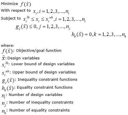
Mathematical Representation of Optimization Problem
In general, optimization problems is decribed in mathemtical form as shown below.:
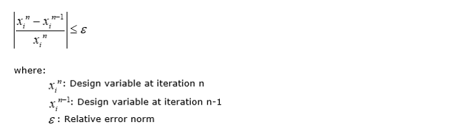
The design variables are updated until the convergence criteria is satisfied. The design variable updates are dependent on sensitivity analysis and step size, where sensitivity analysis and step size will be further discussed in the Design Variable Update section. In order to satisfy such a criteria, the relative difference between the design variables at iterations n and n-1 must be below or equal to the relative error norm. The relative error norm is a user-defined parameter. It is important to note that lower relative norm translates to a higher computing time, as a larger number of iteration is required to satisfy the convergence criteria. However, a higher relative norm decreases the chance of obtaining a globally optimal solution. The relative error norm of 0.0001 is recommended.
Mathematically, the convergence criteria is expressed as follows:
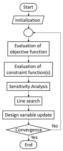
Overall Procedure of Soving Optimization Problem
The generalized workflow for optimization problems is illustrated as below :
As mentioned previously, the design variable update depends on sensitivity analysis and step size. Sensitivity analysis refers to the derivative of objective and constraint functions with respect to the design variables. Gradient-based optimization algorithms evaluate the derivatives analytically, as opposed to using finite differencing methods. Then the gradient search algorithm identifies the search directions based on the sensitivity analysis results, followed by computing the step size for the design variables. The step size defines how far design variables should move along the search directions to decrease the value of the objective function.
The solution to an optimization problem can either converge to a globally or locally optimum solution. Globally optimum solution indicates that the objective function converged to its lowest possible value without constraint violations. On the other hand, locally optimum solution indicates that the objective function converged to its lowest possible value within certain regions of the design variables without constraint violations. As much as global optimum is always desired, it can be particularly difficult to obtain, especially with increased number of design variables and constraint functions. Often times the constraint functions and the initial design variable guesses can prevent the solution from converging to the global optimum. Following plot depicts an example of global and local optimum solutions.
In engineering, most design problems are multidisciplinary in nature, where multiple branches of physics should be considered to design products for performing certain tasks. This led to the rise of the MDO (multidisciplinary design optimization) field, where numerical/analytical optimization techniques are used to design engineering systems. For engineering problems, the constraint functions represent the governing equations from multiple branches of physics. MDO can accelerate the design process by simultaneously considering multiple branches of physics to generate conceptual-level designs that can satisfy various design requirements without manual efforts from engineers and designers. The following process is followed to formulate design optimization problems: 1.Describe the problem: Describe the system that is to be designed, followed by stating the goals and requirements for the system. 2.Gather relevant information: Typically further research is required to quantify all the design requirements. For commercial automotive or aerospace product design problems, this step would involve research in certification requirements. The analysis procedure should also be determined in this stage, and this can involve extraction of governing equations from textbooks and/or literature (e.g. conference and journal papers) or identifications of software tools for performing objective and/constraint function analysis. Furthermore, the set of inputs (i.e. constants) should be defined. 3.Define the design variables: Identify the set of variables that will be updated to develop an optimal design. The lower and/or upper bound of design variables should be quantified based on steps 1 and 2. 4.Define the objective: Derive the mathematical model for the objective function, unless the objective function is to be evaluated using a commercial software. 5.Define the constraints: Derive the mathematical model for all the constraint functions, unless commercial software tools are used to evaluate all the constraint functions. Define the lower and/or upper bounds for the constraint functions.
fmincon() is a built-in function that can be used for solving gradient-based constrained optimization problems using MATLAB and such a function can effectively solve optimization problems with linear and/or non-linear constraints.
The following is the syntax for the built-in function: [x,fval] = fmincon(fun,x0,A,b,Aeq,beq,lb,ub,nonlcon) where: x: Final value of the design variables fval: Final value of the objective function fun: Symbolic equation of the objective function x0: Initial design variable guesses A: Matrix for the coefficients of the linear inequality constraint functions b: Matrix that contains the upper bound of the linear inequality constraint functions Aeq: Matrix for the coefficients of the linear equality constraint functions beq: Matrix for the value of the linear equality constraint functions lb: Matrix that contains the lower bound of the design variables ub: Matrix that contains the upper bound of the design variables nonlcon: Non-linear constraint functions
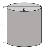
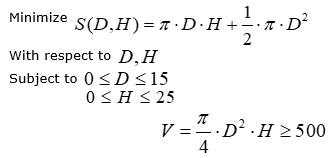
Problem: Design a can that can contain at least 500 mL (1 mL = 1 cm^3) of drink while minimizing the use of a thin aluminum sheet metal (i.e. minimize the surface area of the can). The diameter of the can should not exceed 15 cm and the height of the can should not exceed 25 cm. The lid is also designed using the sheet metal. The can geometry is shown below. The initial guess of the diameter is 12 cm and the height is 21 cm.
Step 1: Formulate the mathematical problem statement
where D is the can diameter and H is the height of the can.
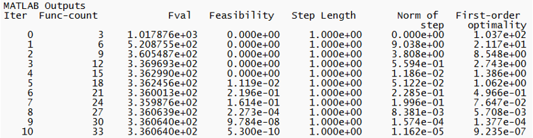
Step 2: MATLAB Implementation
Local minimum found that satisfies the constraints.
Optimization completed because the objective function is non-decreasing in feasible directions, to within the value of the optimality tolerance, and constraints are satisfied to within the value of the constraint tolerance.
<stopping criteria details>
x =
8.4448 8.4448
fval =
336.0640
exitflag =
1
output =
struct with fields:
iterations: 10 funcCount: 33 algorithm: 'sqp' message: '↵Local minimum found that satisfies the constraints.↵↵Optimization completed because the objective function is non-decreasing in ↵feasible directions, to within the value of the optimality tolerance,and constraints are satisfied to within the value of the constraint tolerance.
<stopping criteria details>Optimization completed: The relative first-order optimality measure, 1.740475e-08,↵is less than options.OptimalityTolerance = 1.000000e-06, and the relative maximum constraint↵violation, 5.300080e-10, is less than options.ConstraintTolerance = 1.000000e-06. constrviolation: 5.3001e-10 stepsize: 1.1616e-05 lssteplength: 1 firstorderopt: 9.2350e-07
336.06 cm^3 of aluminum sheet metal is needed to create a can that can contain 473.00 mL of liquid
Reference :
[1]
|
||