PyTorch - Regression

We can use Neural networks for regression by training them on a dataset of input-output pairs. Then, the network learns to map the inputs to the corresponding outputs, allowing it to make predictions on new input data. The network architecture, activation functions, and loss function used for training can all impact the network's ability to perform regression. Popular neural network architectures for regression include feedforward neural networks and convolutional neural networks.

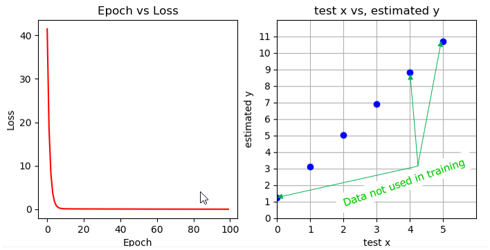
Linear Regression : Single Variable

I used a very simple model as below. This code implements a simple linear regression model using PyTorch. The model is defined as a subclass of the nn.Module class and consists of a single linear layer with one input and one output. The code defines the input and output data as tensors, initializes the model, defines the loss function and optimizer, trains the model for a set number of epochs, and then plots the loss over time and the predicted output for some test input data. The optimization is done using stochastic gradient descent (SGD) with a learning rate of 0.01. The code also uses the matplotlib library to visualize the training process and the predicted output.

import torch

from torch import nn, optim

import matplotlib.pyplot as plt

import numpy as np

 

class LinearRegression_i1_o1(nn.Module):

    def __init__(self):

        super().__init__()

        self.linear = nn.Linear(1,1)

 

    def forward(self,x):

        o = self.linear(x)

        return o

 

x_data = torch.Tensor([[1.0],[2.0],[3.0]]);

y_data = torch.Tensor([[3.0],[5.0],[7.0]]);

 

net = LinearRegression_i1_o1()

 

criterion = nn.MSELoss(reduction='sum')

optimizer = optim.SGD(net.parameters(), lr = 0.01)

 

l = [];

for epoch in range(100):

    y = net(x_data);

    loss = criterion(y,y_data);

    optimizer.zero_grad();

    loss.backward();

    optimizer.step();

    print('epoch = ',epoch, ',' , 'loss = ',loss.item());

    l.append(loss.item());

 

 

x_test = torch.tensor([[0.0],[1.0],[2.0],[3.0],[4.0],[5.0]]);

y = net(x_test);

 

x = x_test.detach().numpy().flatten();

x = list(x);

y = y.detach().numpy().flatten();

y = list(y);

 

plt.subplot(1,2,1);

plt.plot(l,'r-');

plt.title('Epoch vs Loss');

plt.xlabel('Epoch');

plt.ylabel('Loss');

 

plt.subplot(1,2,2);

plt.plot(x,y,'bo');

plt.xlim([0,6]);

plt.ylim([0,12]);

plt.xticks(ticks=range(0,6));

plt.yticks(ticks=range(0,12));

plt.title('test x vs, estimated y');

plt.xlabel('test x');

plt.ylabel('estimated y');

 

plt.grid();

 

plt.show();

 

The result shown are the loss values at each epoch during the training process.

The loss value starts high at the first epoch and gradually decreases over time. As the model is trained on the input data, it learns to better fit the output data and the loss decreases.

At the final epoch, the loss value is very low (0.077), indicating that the model has achieved a good fit to the training data. A low loss value suggests that the model can generalize well to unseen data.

epoch =  0 , loss =  109.12733459472656

epoch =  1 , loss =  48.755165100097656

epoch =  2 , loss =  21.876678466796875

.....

epoch =  96 , loss =  0.08057259768247604

epoch =  97 , loss =  0.07941444963216782

epoch =  98 , loss =  0.078273244202137

epoch =  99 , loss =  0.07714822888374329

 

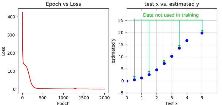
Regression Quadratic Function  : Single Variable

In this example, I will try to fit a simple non-linear data (e.g, quadratic date). The super simple model in previous example would not be able to fit the non-linear data like this. So I needed to revise/expand the model as below.

This code implements a neural network model with two hidden layers to perform regression on a quadratic function. The model is defined as a subclass of the nn.Module class, and it consists of a sequential container with three linear layers separated by sigmoid activation functions. The input and output data are defined as tensors, and the code trains the model using stochastic gradient descent (SGD) with a learning rate of 0.003 and the mean squared error (MSE) loss function.

The code trains the model for 2000 epochs and prints the loss value every 100 epochs. After training, the code evaluates the model on some test data and plots the loss over time and the predicted output for the test data.

The model is capable of learning a quadratic function as the input-output relationship, which is a more complex function than the simple linear regression model. Therefore, the loss value starts higher and takes longer to converge to a lower value. The plot of the predicted output shows that the model has learned the quadratic relationship between the input and output data.

import torch

from torch import nn, optim

import matplotlib.pyplot as plt

import numpy as np

 

class Regression_Quad_i1_h2_o1(nn.Module):

    def __init__(self):

        super().__init__()

        self.net = nn.Sequential(

                                nn.Linear(1,4),

                                nn.Sigmoid(),

                                nn.Linear(4,6),

                                nn.Sigmoid(),

                                nn.Linear(6,1)

                                );

 

    def forward(self,x):

        o = self.net(x)

        

        return o

 

x_data = torch.Tensor([[1.0],[2.0],[3.0],[4.0]]);

y_data = torch.Tensor([[1.0],[5.0],[10.0],[17.0]]);

 

net = Regression_Quad_i1_h2_o1()

 

criterion = nn.MSELoss(reduction='sum')

optimizer = optim.SGD(net.parameters(), lr = 0.003)

 

l = [];

for epoch in range(2000):

    y = net(x_data);

    loss = criterion(y,y_data);

    optimizer.zero_grad();

    loss.backward();

    optimizer.step();

    if (epoch % 100) == 0:

        print('epoch = ',epoch, ',' , 'loss = ',loss.item());

    l.append(loss.item());

 

 

x_test = torch.tensor([[0.0],[0.5],[1.0],[1.5],[2.0],[2.5],[3.0],[3.5],[4.0],[5.0]]);

#x_test = torch.tensor(np.linspace(0,5,10));

#x_test = x_test.view(10,1);

y = net(x_test);

 

x = x_test.detach().numpy().flatten();

x = list(x);

y = y.detach().numpy().flatten();

y = list(y);

 

plt.subplot(1,2,1);

plt.plot(l,'r-');

plt.title('Epoch vs Loss');

plt.xlabel('Epoch');

plt.ylabel('Loss');

 

plt.subplot(1,2,2);

plt.plot(x,y,'bo');

plt.xlim([0,6]);

plt.ylim([-5,30]);

plt.xticks(ticks=range(0,6));

plt.yticks(ticks=range(-5,30,5));

plt.title('test x vs, estimated y');

plt.xlabel('test x');

plt.ylabel('estimated y');

 

plt.grid();

 

plt.show();

 

The loss values shown in the result below start high and decrease over time, indicating the model is learning the input-output relationship. The loss reaches a minimum at epoch 900, suggesting good model performance. The predicted output shows that the model accurately learned the quadratic relationship between input and output data.

epoch =  0 , loss =  459.1344909667969

epoch =  100 , loss =  115.44194030761719

epoch =  200 , loss =  35.4473762512207

epoch =  300 , loss =  6.033346652984619

epoch =  400 , loss =  2.90378737449646

epoch =  500 , loss =  2.3812389373779297

epoch =  600 , loss =  2.0026025772094727

epoch =  700 , loss =  1.609250545501709

epoch =  800 , loss =  1.264915108680725

epoch =  900 , loss =  1.0008598566055298

epoch =  1000 , loss =  1.4073749780654907

epoch =  1100 , loss =  1.5786477327346802

epoch =  1200 , loss =  1.4552806615829468

epoch =  1300 , loss =  1.2912174463272095

epoch =  1400 , loss =  1.1246427297592163

epoch =  1500 , loss =  0.9764596819877625

epoch =  1600 , loss =  0.8541290163993835

epoch =  1700 , loss =  0.7479215264320374

epoch =  1800 , loss =  0.6534777879714966

epoch =  1900 , loss =  0.5714238882064819