In this note, I will try with completely different approach that I used in other note. Now with chatGPT available at our hand, I think the way we learn new things (including programming language). For general approach that I take in terms of learning a programming using chatGPT, I wrote a separte note titled Learn From chatGPT.
In addition, we can find a lot of YouTube video that can explain the conceptual things much better than I do. So I would not try to explain any conceptual things (unless I really think it is necessary) or try to explain about syntax of the code. You can easily find a YouTube about the concept (check out the video under YouTube section in this note) or you can ask it to chatGPT.
What I am going to do in this note is to show how I am learning the basic concept of RNN from chatGPT. Just follow through my chat with chatGPT and hope it is helpful with you as well. Followings are the details of chatGPT and python that I have used for this note.
- Date : Apr 9, 2023
- chatGPT : GPT 4
- Python : Python 3.8.10
- pyTorch : 1.13.1+cpu
This is my first request :
|
Write an example of RNN network for time series data prediction in pytorch. Use an imaginary data for the test |
This is the code. The first code worked without any debugging.
|
RNN_01.py |
|
import numpy as np import matplotlib.pyplot as plt
import torch import torch.nn as nn import torch.optim as optim
from sklearn.preprocessing import MinMaxScaler from sklearn.metrics import mean_squared_error
# Generate a sine wave dataset with Gaussian noise t = np.arange(0, 100, 0.1) noise = np.random.normal(0, 0.1, t.shape) df = (np.sin(t) + noise).reshape(-1, 1)
# Hyperparameters input_size = 1 hidden_size = 32 num_layers = 2 output_size = 1 sequence_length = 30 num_epochs = 100 learning_rate = 0.01
# Normalize data scaler = MinMaxScaler(feature_range=(-1, 1)) data = scaler.fit_transform(df)
# Train-test split train_data = data[:int(data.shape[0]*0.8)] test_data = data[int(data.shape[0]*0.8)-sequence_length:]
# Create sliding window data def sliding_windows(data, seq_length): x = [] y = [] for i in range(len(data)-seq_length-1): _x = data[i:(i+seq_length)] _y = data[i+seq_length] x.append(_x) y.append(_y) return np.array(x), np.array(y)
trainX, trainY = sliding_windows(train_data, sequence_length) testX, testY = sliding_windows(test_data, sequence_length)
# Convert to torch tensors trainX = torch.tensor(trainX).float() trainY = torch.tensor(trainY).float() testX = torch.tensor(testX).float() testY = torch.tensor(testY).float()
class RNN(nn.Module): def __init__(self, input_size, hidden_size, num_layers, output_size): super(RNN, self).__init__() self.hidden_size = hidden_size self.num_layers = num_layers self.rnn = nn.RNN(input_size, hidden_size, num_layers, batch_first=True) self.fc = nn.Linear(hidden_size, output_size)
def forward(self, x): h0 = torch.zeros(self.num_layers, x.size(0), self.hidden_size) out, _ = self.rnn(x, h0) out = self.fc(out[:, -1, :]) return out
model = RNN(input_size, hidden_size, num_layers, output_size)
criterion = nn.MSELoss() optimizer = optim.Adam(model.parameters(), lr=learning_rate)
# Training loop for epoch in range(num_epochs): outputs = model(trainX) optimizer.zero_grad() loss = criterion(outputs, trainY) loss.backward() optimizer.step()
if (epoch+1) % 10 == 0: print(f'Epoch [{epoch+1}/{num_epochs}], Loss: {loss.item():.4f}')
# Evaluate the model model.eval() test_outputs = model(testX) test_outputs = test_outputs.detach().numpy() testY = testY.numpy()
# Invert the scaling to original values test_outputs = scaler.inverse_transform(test_outputs) testY = scaler.inverse_transform(testY)
# Calculate RMSE rmse = np.sqrt(mean_squared_error(testY, test_outputs)) print(f"RMSE: {rmse:.4f}")
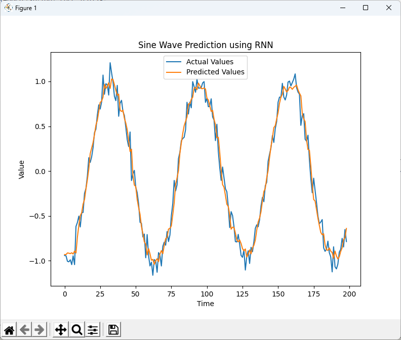
# Plot the results plt.figure(figsize=(12, 6)) plt.plot(testY, label='Actual Values') plt.plot(test_outputs, label='Predicted Values') plt.legend() plt.xlabel("Time") plt.ylabel("Value") plt.title("Sine Wave Prediction using RNN") plt.show() |
| Result |
|
Epoch [10/100], Loss: 0.0342 Epoch [20/100], Loss: 0.0150 Epoch [30/100], Loss: 0.0128 Epoch [40/100], Loss: 0.0115 Epoch [50/100], Loss: 0.0109 Epoch [60/100], Loss: 0.0104 Epoch [70/100], Loss: 0.0098 Epoch [80/100], Loss: 0.0095 Epoch [90/100], Loss: 0.0094 Epoch [100/100], Loss: 0.0092 RMSE: 0.1128 |
|
|
Challenging against RNN with random data
I wanted to give some hard time to give this model and requested as follows.
|
can you give me an example data that make it difficult to predict with RNN ? |
chatGPT gave me different test data.
|
RNN_01.py |
|
#same as before
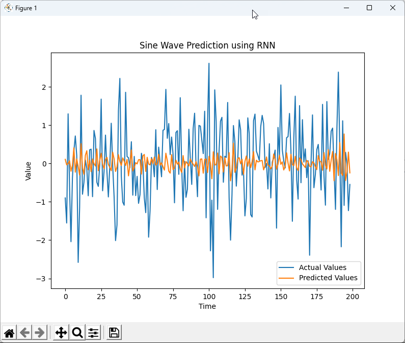
# Generate a sine wave dataset with Gaussian noise t = np.arange(0, 100, 0.1) df = np.random.randn(t.shape[0]).reshape(-1, 1)
# same as before |
As you see below, chatGPT did pretty good job giving hard time to the model.
| Result |
|
Epoch [10/100], Loss: 0.1170 Epoch [20/100], Loss: 0.1109 Epoch [30/100], Loss: 0.1104 Epoch [40/100], Loss: 0.1101 Epoch [50/100], Loss: 0.1096 Epoch [60/100], Loss: 0.1091 Epoch [70/100], Loss: 0.1088 Epoch [80/100], Loss: 0.1087 Epoch [90/100], Loss: 0.1086 Epoch [100/100], Loss: 0.1084 RMSE: 1.0634 |
|
|
Then another question popped up in my mind. I was wondering if the poor performance is due to the nature of RNN itself or due to the specific model and hyperparameters used in the specific example used above. Now... just follow through the QnA between me and chatGPT.
|
can you explain why this data is hard to predict with RNN ? Is it because of the nature of RNN ? or Hyperparameters you set in this example ? |
Reply from chatGPT :
|
The difficulty in predicting this data using an RNN is primarily due to the nature of the data itself. The dataset we generated with np.random.randn consists of random samples from a standard normal distribution. This means that the data has no discernible underlying structure or pattern, making it difficult for an RNN or any other model to capture any useful information for making accurate predictions. RNNs are well-suited for time series prediction tasks that have some structure or temporal dependencies, as they can maintain hidden states to capture information from previous time steps. However, when the data is purely random and lacks any meaningful structure, the RNN will struggle to learn from the data and make accurate predictions. The hyperparameters in the example provided earlier are relatively simple and may not be optimal for more complex datasets, but the primary reason for the poor performance on this specific dataset is the lack of structure in the data itself. Even if you were to optimize the hyperparameters or use more advanced models like LSTMs or GRUs, predicting purely random data accurately would remain a challenging task. |
|
If it sounds as if it is due to the Nature of RNN and the nature of data (pure random with no inherent structure), right ? |
Reply from chatGPT :
|
Yes, that's correct. The difficulty in predicting the purely random data accurately is due to both the nature of the data (having no inherent structure) and the nature of RNNs. Since the data lacks any meaningful structure or temporal dependencies, RNNs (as well as other models) will struggle to learn any useful information for making accurate predictions. RNNs are designed to capture and learn from the structure or temporal dependencies in time series data. When the data is purely random, the ability of RNNs to maintain hidden states and capture information from previous time steps does not provide any advantage, as there's no pattern to learn. To summarize, the primary reason for the difficulty in predicting this random dataset is the lack of structure in the data itself. While the nature of RNNs also contributes to the challenge, even more advanced models like LSTMs or GRUs would have trouble predicting purely random data accurately. |
|
Is there any Deep learning model that can work even with this kind of data ? |
Reply from chatGPT :
|
Predicting purely random data accurately is inherently challenging for any machine learning model, including deep learning models. The primary reason is that machine learning models, including deep learning models, learn patterns and structures in the data to make predictions. If the data is purely random and lacks any meaningful structure or pattern, there's no information for the model to learn and leverage for making accurate predictions. While some deep learning models like LSTMs, GRUs, or attention mechanisms might perform better than a simple RNN in capturing more complex temporal dependencies, they would still struggle to predict purely random data accurately. It's essential to understand that the effectiveness of any machine learning or deep learning model depends on the presence of patterns or structure in the data. If the data is purely random, it's unlikely that any model will be able to make accurate predictions. In practice, real-world time series data often contains some level of structure or pattern, even if it's noisy or non-stationary, which can be leveraged by deep learning models for better predictions. |
Challenging against RNN with synthetic data
The problem in previous section may not be purely because of RNN, it would be largely because of the nature of data itself. Since the data is purely random data with no internal structure. So I asked chatGPT to generate a synthetic data that would challenge against the RNN.
chatGPT gave me different test data.
|
RNN_01.py |
|
#same as before
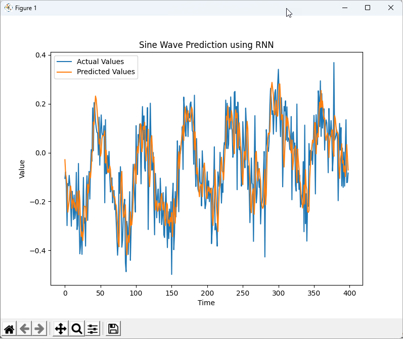
# Generate a time series with more complex structure, damping, and non-linearity t = np.arange(0, 200, 0.1) damping = np.exp(-t / 100)
df = (damping * (np.sin(t) + 0.5 * np.sin(t / 10) + 0.25 * np.sin(2 * t) + 0.1 * np.sin(3 * t) + 0.5 * np.sin(t / 20) * np.sin(t / 15) + 0.1 * np.sin(t / 5)**2 + 0.15 * np.sin(t / 8) * np.sin(t / 12) * np.sin(t / 20)))
# same as before |
As you see below, chatGPT did pretty good job giving hard time to the model.
| Result |
|
Epoch [10/100], Loss: 0.0225 Epoch [20/100], Loss: 0.0100 Epoch [30/100], Loss: 0.0105 Epoch [40/100], Loss: 0.0079 Epoch [50/100], Loss: 0.0078 Epoch [60/100], Loss: 0.0075 Epoch [70/100], Loss: 0.0072 Epoch [80/100], Loss: 0.0071 Epoch [90/100], Loss: 0.0070 Epoch [100/100], Loss: 0.0069 RMSE: 0.1276 |
|
|
It was not easy to synthetically generate challenging data. So I decided to try with real data as described in next section.
Challenging against RNN with real life data (Stock Price Data)
I wanted to give some hard time to give this model and requested as follows.
|
can you use the data from a csv file for the training of the RNN code that you provided ? the data format is as follows. You can use panda if you like. date open high low close volume Name 2014-03-27 568 568 552.92 558.46 13052 GOOG 2014-03-28 561.2 566.43 558.67 559.99 41003 GOOG 2014-03-31 566.89 567 556.93 556.97 10772 GOOG 2014-04-01 558.71 568.45 558.71 567.16 7932 GOOG 2014-04-02 565.106 604.83 562.19 567 146697 GOOG 2014-04-03 569.85 587.28 564.13 569.74 5087530 GOOG 2014-04-04 574.65 577.77 543 543.14 6377658 GOOG 2014-04-07 540.74 548.48 527.15 538.15 4389569 GOOG 2014-04-08 542.6 555 541.61 554.9 3152406 GOOG |
chatGPT gave me different test data.
|
RNN_04.py |
|
import pandas as pd import numpy as np import torch import torch.nn as nn from torch.autograd import Variable import matplotlib.pyplot as plt from sklearn.preprocessing import MinMaxScaler
# Read the data from the CSV file df = pd.read_csv('C:\\RyuCloud\\Python\\StockData\\individual_stocks_5yr\\A_data.csv', index_col='date')
# Extract the closing prices closing_prices = df['close'].values.reshape(-1, 1)
# Normalize the closing prices between 0 and 1 scaler = MinMaxScaler(feature_range=(0, 1)) closing_prices = scaler.fit_transform(closing_prices)
# Split the data into training and testing sets train_size = int(len(closing_prices) * 0.8) train_set = closing_prices[:train_size] test_set = closing_prices[train_size:]
# Create sequences and targets for training and testing def create_sequences(data, seq_length): inputs = [] targets = []
for i in range(len(data) - seq_length - 1): inputs.append(data[i:i+seq_length]) targets.append(data[i+seq_length])
return np.array(inputs), np.array(targets)
seq_length = 100 train_inputs, train_targets = create_sequences(train_set, seq_length) test_inputs, test_targets = create_sequences(test_set, seq_length)
# Convert the inputs and targets to PyTorch tensors train_inputs = Variable(torch.Tensor(train_inputs)) train_targets = Variable(torch.Tensor(train_targets)) test_inputs = Variable(torch.Tensor(test_inputs)) test_targets = Variable(torch.Tensor(test_targets))
# Define the RNN model class RNN(nn.Module): def __init__(self, input_size, hidden_size, output_size): super(RNN, self).__init__() self.rnn = nn.RNN(input_size, hidden_size, batch_first=True) self.linear = nn.Linear(hidden_size, output_size)
def forward(self, x, hidden): x, hidden = self.rnn(x, hidden) x = self.linear(x.squeeze(1)) return x, hidden
# Set up the RNN model and training parameters input_size = 1 hidden_size = 128 #64 output_size = 1 num_epochs = 100 learning_rate = 0.001
model = RNN(input_size, hidden_size, output_size) criterion = nn.MSELoss() optimizer = torch.optim.Adam(model.parameters(), lr=learning_rate)
# Train the RNN model for epoch in range(num_epochs): hidden = Variable(torch.zeros(1, train_inputs.size(0), hidden_size))
outputs, _ = model(train_inputs, hidden) optimizer.zero_grad()
loss = criterion(outputs.squeeze(2), train_targets) loss.backward()
optimizer.step()
if (epoch + 1) % 10 == 0: print(f'Epoch [{epoch + 1}/{num_epochs}], Loss: {loss.item():.4f}')
# Test the RNN model model.eval() test_hidden = Variable(torch.zeros(1, test_inputs.size(0), hidden_size)) test_outputs, _ = model(test_inputs, test_hidden) test_loss = criterion(test_outputs.squeeze(2), test_targets) print(f'Test Loss: {test_loss.item():.4f}')
# Use the last sequence in the test set to make a prediction last_sequence = test_inputs[-1:] last_sequence = Variable(last_sequence) last_hidden = Variable(torch.zeros(1, last_sequence.size(0), hidden_size)) pred, _ = model(last_sequence, last_hidden) pred = pred.data.numpy().reshape(-1, 1) pred = scaler.inverse_transform(pred)
print(f'Next predicted closing price: {pred[0][0]:.4f}')
# Plot the test predictions test_outputs = test_outputs.data.numpy() test_targets = test_targets.numpy() test_outputs = scaler.inverse_transform(test_outputs.reshape(-1, 1)).flatten() test_targets = scaler.inverse_transform(test_targets.reshape(-1, 1)).flatten()
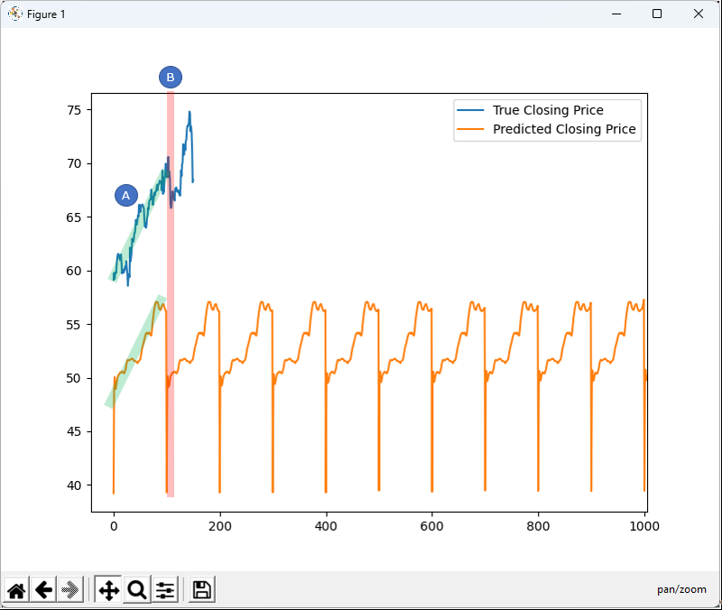
plt.figure(figsize=(10, 3)) plt.plot(test_targets, label='True Closing Price') plt.plot(test_outputs, label='Predicted Closing Price') plt.legend() plt.show() |
As you see below, chatGPT did pretty good job giving hard time to the model.
| Result |
|
Epoch [10/100], Loss: 0.0365 Epoch [20/100], Loss: 0.0260 Epoch [30/100], Loss: 0.0210 Epoch [40/100], Loss: 0.0151 Epoch [50/100], Loss: 0.0141 Epoch [60/100], Loss: 0.0138 Epoch [70/100], Loss: 0.0135 Epoch [80/100], Loss: 0.0134 Epoch [90/100], Loss: 0.0134 Epoch [100/100], Loss: 0.0134 |
|
|
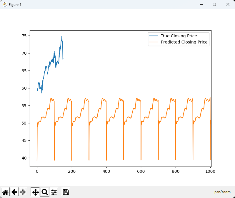
At the first glimpse, you would notice that prediction is very poort. Looking further into details, the initial trending (marked as (A)) went relatively OK but it went to complete failure when sudden drop happens (marked as (B))
I wanted to understand the limitation of RNN using this example and went on some Q&A with chatGPT.
|
with RNN, the prediction gets so poor when the training data changes abruptly. for example, the data drops abruptly, the predicted data seriously undershoot. Would this be due to the nature of RNN ? |
Reply from chatGPT :
|
RNNs can indeed have difficulty modeling abrupt changes in time series data, such as sudden drops or spikes. This issue can be attributed to a few factors:
Using more advanced recurrent models, like Long Short-Term Memory (LSTM) networks or Gated Recurrent Unit (GRU) networks, can help mitigate these issues. These models are specifically designed to address the vanishing gradient problem and improve the model's ability to learn long-term dependencies. They may provide better performance in situations where the data contains abrupt changes. Another option is to explore other types of models, such as attention-based models like the Transformer, or even hybrid models that combine convolutional layers with recurrent layers. Additionally, it's essential to preprocess the data and engineer relevant features effectively. In some cases, incorporating external factors, such as news sentiment or macroeconomic indicators, can help improve the model's ability to capture abrupt changes in the data. |
|
would changing seq_length make any improvement ? |
Reply from chatGPT :
|
Changing the seq_length can have an impact on the model's performance, but whether it will lead to an improvement depends on the specific problem and dataset. The seq_length represents the number of time steps the model considers when making predictions, which determines how much past information the model can use.
To determine the optimal seq_length, you can perform experiments with different values and evaluate the model's performance using cross-validation or a validation set. Keep in mind that the optimal seq_length might depend on the specific problem, dataset, and model architecture. It's also worth noting that if you're using a vanilla RNN, increasing the seq_length too much could exacerbate the vanishing gradient problem. In such cases, consider using more advanced recurrent models like LSTMs or GRUs, which are better equipped to handle longer sequences and learn long-term dependencies. |
|
Is there any hyper parameter for RNN to relieave 'Short-term memory' problem at least to some degree ? |
Reply from chatGPT :
|
The 'short-term memory' problem in RNNs is primarily due to the vanishing gradient problem, which makes it difficult for the network to capture long-term dependencies in the data. While there isn't a specific hyperparameter that can directly relieve this problem, you can consider the following strategies to improve RNN's ability to model longer-term dependencies:
Keep in mind that these strategies may help improve the RNN's ability to capture long-term dependencies to some degree, but they may not completely solve the short-term memory problem. LSTMs and GRUs are generally more effective at handling sequences with long-term dependencies than vanilla RNNs. |
YouTube
- What is Recurrent Neural Network (RNN)? Deep Learning Tutorial 33 (Tensorflow, Keras & Python) - codebasics(2021)
- Types of RNN | Recurrent Neural Network Types | Deep Learning Tutorial 34 (Tensorflow & Python) - codebasics(2021)
- Vanishing and exploding gradients | Deep Learning Tutorial 35 (Tensorflow, Keras & Python) - codebasics(2021)
- Simple Explanation of LSTM | Deep Learning Tutorial 36 (Tensorflow, Keras & Python) - codebasics(2021)
- Recurrent Neural Networks (RNNs), Clearly Explained!!! - StatQuest with Josh Starmer (2022)
- [혁펜하임 X 테디노트] 왜 RNN보다 트랜스포머가 더 좋다는 걸까? - TeddyNote (2024)