Filter is a components that selectively pass "what it likes" and block "what it dislike". When we are talking about the characteristics of filter, we usually describe it in frequency domain.

This page starts with the four basic filter shapes and the numbers used to specify them. Then it compares the ideal shape with the responses that can actually be built. After that it looks at the main technologies used to build a filter, and it ends with the three properties every filter designer tries to improve.

• What are the four basic filter types ?
• Ideal vs Real filter
• Typical Implementation of a Filter
• Design Goal

What are the four basic filter types ?

In most case, a filter would belong to one of the four possible ideal types as shown below(There can be some other variations of filter, e.g, a filter with multiple pass bands etc, but more than 99% of filters you can see would be one of the following types).

Each of the four plots below draws amplitude against frequency. The green area marks the range the filter should pass, and the red line is the ideal filter response.

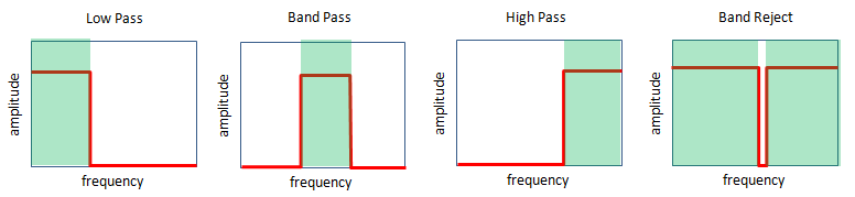
The four ideal filter types. Each one is defined only by which part of the frequency axis it passes.

• Low Pass: the red line stays high from zero frequency up to the edge of the green area, then drops to zero.
• Band Pass: the red line is high only inside a green block in the middle of the axis.
• High Pass: the red line is zero at low frequency and rises at the start of the green area on the right.
• Band Reject: the green area covers almost the whole axis, and the red line drops only in a narrow gap in the middle.

Low pass filter is a filter that passes the signal with low frequecy and blocks high frequency signal. How low the frequency should be is dependent on the specification of the filter.

High pass filter is a filter that passes the signal with high frequecy and blocks low frequency signal. How high the frequency should be is dependent on the specification of the filter.

Band pass filter is a filter that passes a certain range of frequency and blocks both lower and higher region than the specificied range. The frequency range that passes the filter is determined by the specification.

Band Reject filter is a filter that passes most of the frequency except a very narrow range of the frequncy. The purpose of the other types of the filter is to pass signals with a certain range, but the purpose of the band reject filter is to block a selected frequency of the signal.

A band reject filter with a very narrow stopband is also called a notch filter. A wider band reject filter is possible too, for example one that blocks a whole transmit band next to a receive band.

The ideal shapes above hide one question: where exactly does the passband end? A real response has no vertical edge, so the edge is defined by a level. The usual choice is the cutoff frequency, where the response has fallen 3 dB below its passband level. At that point the filter passes half of the input power, because 10 x log₁₀(0.5) is -3.01 dB. A band pass filter has two cutoff frequencies, and the distance between them is its 3 dB bandwidth.

A filter datasheet describes the response with a handful of numbers. The table below lists the ones you will meet most often, and the rest of this page comes back to each of them.

• A filter type is defined by its passband : low pass, high pass, band pass and band reject differ only in which frequency range they pass.
• The cutoff frequency is a 3 dB point : a real response has no vertical edge, so the half power point marks where the passband ends.
• A filter is specified by several numbers : insertion loss, ripple, stopband attenuation, transition band, return loss and group delay together describe how close it is to the ideal.

Ideal vs Real filter

Ideal filter is the filter as illustrated above. It passes a certain range of the signal and start blocking the signal right next to the range. But as I always say, there is no device which act like ideal concept. Same in filter as well.

Let's look into a bandpass filter as an example. The ideal filter that everybody wants to have is the one as shown on the left, but you would never get this kind of filter. Even in theoretical design of a filter, you would see several types as shown in the middle colum but even this theoretical filter is not as good as the ideal filter.

The first theoretical type has some fluctuations (ripples) in the passband area and relatively steeply fall into the blocking area (stop band) and does not have fluctuations in the stopband.

The second theoretical type does not have ripples either passband nor in stop band. No ripple is very good.. but in this type it slowly falls into the blocking area.

The third theoretical type has ripples both in pass band and stop band which is not good, but it falls into stop band very steeply which is good.

Some of examples of real filter are shown on the right column, which is obviously worse than the theoretical properties. These are only a couple of real filter.. in real world you woud have much diverse type and characteristics of filters.

The picture below puts the three kinds of band pass response side by side. The ideal response is on the left, three theoretical responses are in the middle, and three measured responses are on the right.

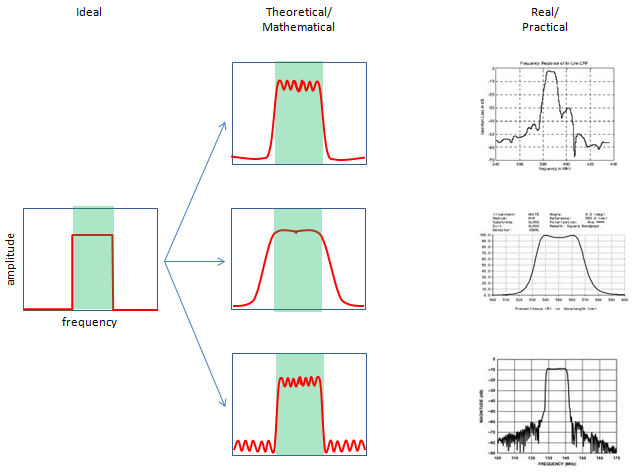
Ideal, theoretical and real band pass responses. Every theoretical response trades ripple against steepness, and a real filter adds loss and spurious peaks on top of that.

• Ideal: a rectangle over the green passband, with amplitude on the vertical axis and frequency on the horizontal axis.
• Theoretical, top: ripple inside the passband, steep edges and a flat stopband.
• Theoretical, middle: no ripple and slow, rounded edges. The small dip drawn at the top is part of the sketch, because this response is flat at the centre of the passband.
• Theoretical, bottom: ripple in the passband and in the stopband, and the steepest edges of the three.
• Real, top: a plot titled Frequency Response of In-Line CRF. It shows insertion loss in dB from 340 to 440 MHz, with a peak near 385 MHz and an uneven stopband between about -30 and -65 dB.
• Real, middle: a transmittance plot in percent against wavelength from 500 to 600 nm. It comes from an optical square band pass filter, so it shows the shape rather than an RF measurement.
• Real, bottom: magnitude in dB from 105 to 175 MHz. The passband runs from about 130 to 145 MHz at about -10 dB, and the stopband is noisy at about -60 to -80 dB.

The three theoretical responses have standard names. The top one, with ripple only in the passband, is the Chebyshev type I response. The middle one, with no ripple anywhere, is the Butterworth response. It is also called maximally flat. The bottom one, with ripple in both bands, is the elliptic response, also called the Cauer response.

Two more names are common. A Chebyshev type II response puts the ripple in the stopband and keeps the passband flat. A Bessel response has an even slower transition than Butterworth, but its phase is almost linear. So Bessel is the choice when the waveform shape matters more than the rejection, which connects to the phase linearity goal in Design Goal below.

How much steeper is each response for the same order ?

The order of a filter is the number of reactive elements, or poles, in its design. More order gives a steeper transition but costs size and loss. So let's fix one requirement and see how much order each response needs to meet it.

Take a low pass requirement with at most 1 dB of loss at the passband edge f_p and at least 40 dB of attenuation at 2 x f_p. The minimum orders below were computed with the standard order formulas for analog prototypes.

You can also look at it from the other side and fix the order. With order 5, a Butterworth low pass gives 30.1 dB of attenuation at twice its 3 dB cutoff. A Chebyshev type I with 1 dB of ripple gives 45.3 dB at twice its ripple bandwidth edge, and a Bessel filter gives only 14.1 dB. The Butterworth number follows a simple rule: far from the cutoff, the response falls by 20 x N dB per decade, or about 6 x N dB per octave, where N is the order.

• The theoretical responses have names : Chebyshev type I, Butterworth and elliptic are the three drawn above, and Chebyshev type II and Bessel are two more.
• Ripple buys steepness : an elliptic filter meets the example requirement with order 4, where Butterworth needs order 8.
• A flat and steep filter costs order : every extra order adds components, size and insertion loss to a real filter.
• A real filter is worse than its theory : the measured plots show extra loss, uneven stopbands and spurious peaks that the prototype does not have.

Typical Implementation of a Filter

There are so many different ways to implement a filter and it would be difficult to list all of possible ways of filter implementation method. I will just list several ways of implementation which I think are most commonly used in many area. Followings are some examples of filter implementation.

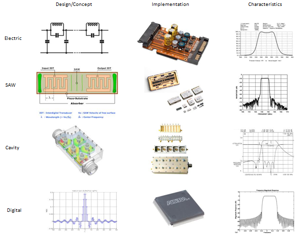
Four ways to build a filter. Each row shows the design idea, a real part and a typical response.

• The rows are Electric, SAW, Cavity and Digital. The columns are Design/Concept, Implementation and Characteristics.
• Electric: an LC ladder with shunt capacitors and parallel LC pairs in the series arms. The response plot in this row is the optical transmittance curve against wavelength, so read it only as a generic band pass shape.
• SAW: an Input IDT and an Output IDT on a Piezo-Substrate, with an absorber at each end. The legend defines IDT as Interdigital Transducer and gives the wavelength as λ = Vo/f0, where Vo is the SAW velocity of free surface and f0 is the center frequency.
• Cavity: a metal housing with resonator posts inside, a set of cavity filter units, and an analyzer screen with an attenuation trace and a frequency response trace.
• Digital: an impulse response h(n) shaped like a sinc function, an FPGA chip, and a magnitude response in dB against normalized frequency.

Electrical Filter : This is a method to implement a filter using basic electrical components (e.g,R/L/C) and I think this would be the most common and widely used filter type. Depending on application, only a single component like single Inductor or single capcitor can be a filter and in some other applications you will see very complicated combinations of these component which functions as a filter.

The parallel LC pairs in the ladder drawing are not decoration. Each pair resonates at one frequency and blocks it completely, which puts a notch in the stopband. Those notches are how an elliptic response gets its stopband ripple.

SAW Filter (Surface Acoustic Wave Filter) : This is a type of filter which converts electrical energy into an acoustic energy and apply filtering and then convert the filtered energy back into electrical energy. Adavantage of this type of filter is that it can implement very high quality (very high order filter) in relatively small size. Disadvantage of this type would be that it is hard to handle high power and it generally cause large insertion loss. In most of mobile phone, you would see at least one or two SAW filter mostly in RF stage. They used to use SAW filter in IF stage as well, but now in most mobile phone the whole IF stage is gone and so is the IF SAW filter.

The small size of a SAW filter comes from the slow speed of the acoustic wave. The wavelength in the IDT is λ = Vo/f0, and Vo is a few thousand m/s on common piezoelectric substrates. For example, with Vo = 4000 m/s, a 1 GHz filter has an acoustic wavelength of 4 micrometers. The electromagnetic wavelength at 1 GHz in free space is 30 cm, which is 75000 times longer. So a structure that is many wavelengths long still fits on a small chip.

Cavity Filter : When I saw this type of filter I was amazed by the fact that such a simple bulky metalic object can act as a filter. (Internal structure is not as simple as I thought, but at least from outlook it just looked like a metalic chunk -:). In terms of filter characteristics, I would not call it very high performance, but it can handle very high power and the frequency range it can cover can reach up to extremly high frequency and the insertion loss is usually very small compared to other types of filter.

Digital Filter :

Digital Filter : As you may guess, it is a type of filter which perform filtering based on numerical algorithm. To use this filter, first you have to convert the incoming analog signal into digital signal and then process the digitized data. The advatage of this type of filter would be that you can get the filter performance which is almost same as you designed in theory. The disadvantage would be that it would be difficult to handle high frequency mainly due to the limitation of AD converter sampling rate. Of course, you can downconvert the high frequenty to low frequency so that you can use digital filter, but it means you would need additional circuit for filtering. Another disadvantage would be that it would cause relatively long delay due to the delay caused by each digital gate component.

For the delay, the main cause is the filter itself rather than the gates. A linear phase FIR filter with N taps delays every signal by (N - 1)/2 samples. For example, a 101 tap filter running at 30.72 MHz delays the signal by 50 samples, which is about 1.63 microseconds. The ADC, the DAC and any sample rate conversion add their own delay on top of that.

• An LC filter is the general solution : it works from low frequency to microwave, and its order is set by the number of L and C elements.
• A SAW filter is small because sound is slow : the acoustic wavelength is about five orders of magnitude shorter than the radio wavelength at the same frequency.
• A cavity filter handles power : it is large, but it has low loss and can take the power of a base station transmitter.
• A digital filter is exact but late : it follows its design almost perfectly, but it needs an ADC and adds a delay of (N - 1)/2 samples for a linear phase FIR.

Design Goal

Once the filter type and the technology are chosen, the designer still has to balance three properties. Improving one of them usually costs another one, so it helps to name them before looking at any design.

Regardless of what kind of filter you want to design, the basic design goal would all be same as illustrated below.

(1) Steep Transition Phase : The first and the most important characteristics you want to achieve would be the transition phase as sharp as possible as marked by (1). Everybody want to improve this property from the solid line to the dotted line. Usually we increase the order of the filter to achieve this, but this order increment would make the filter bigger or complicated. In case of passive filter, this order increment would cause large insertion loss as well.

One of filters with steepest transition phase without increasing the size too much would be 'SAW' filter, but Insertion Loss of SAW filter is relatively large comparing to other types of filters. Especially IF SAW filter has extremely sharp transition but super large insertion loss.

(2) Small Insertion Loss : Needless to day, everybody wants to have the insertion loss as small as possible, but it is not easy to improve the insertion loss, especially when the loss is caused by the material property of the filter (e.g, SAW filter).

Insertion loss is easier to feel as a ratio. A filter with 1 dB of insertion loss passes 79.4 % of the power, and a filter with 3 dB passes 50.1 %. In a receiver the loss also matters for noise. A passive filter at room temperature has a noise figure equal to its insertion loss. So a 2 dB filter in front of an LNA with a 1 dB noise figure gives a total noise figure of 3 dB.

(3) Phase Linearity : Everybody want to have non-changing or at least linear phase characteristics across the passband region as shown in dotted line, but in reality most of the filter would have the fluctuating, sometimes even more complicated phase characteristics. Unfortunately it is extremely difficult to optimize the phase characteristics.

The phase goal is easier to read as group delay. The group delay is τ = -dφ/dω, the negative slope of the phase against angular frequency. A linear phase gives a constant group delay, so every frequency component arrives with the same delay and the waveform keeps its shape. A phase that bends near the band edges gives a larger delay there, and a wideband signal is distorted. This is why the Bessel response and the linear phase FIR filter are used when the waveform shape matters.

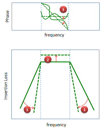
The three filter design goals. The solid lines are a typical filter, and the dashed lines are the target.

• Bottom plot: the vertical axis is labelled Insertion Loss, but the curve is drawn as the passed signal level. So a higher line means less insertion loss.
• Marker 1 appears on both edges of the bottom plot. The curved red arrows turn the solid sloped edges into the steeper dashed edges.
• Marker 2 sits on the top of the passband. The red arrow moves the solid top up to the dashed line, which is the smaller insertion loss.
• Top plot: the phase against frequency. The solid curves wander inside the passband, and the dashed straight lines show a flat and a linear phase. Marker 3 and its red arrow point from the wavy curve to the straight line.

• Steepness costs order : a steeper transition needs a higher order, and a higher order makes a passive filter bigger and more lossy.
• Insertion loss adds directly to noise figure : in front of an LNA, every dB of filter loss is a dB of receiver noise figure.
• Phase linearity means constant group delay : a constant delay keeps the waveform shape, and a bending phase near the band edges distorts a wideband signal.