Characteris Impendance is one of the terms we see the most often and use ourselves, but very vague and hard to explain. Following is some of the definition of Characteristic Impendance from several different sources. (If you check 10 different sources, you would see 10 different variations of description).

The definitions are quoted in the first section below. After them, this page builds the idea step by step with a thought experiment: a source, a meter, and a line that first ends open, then runs forever, and finally ends in a load. The last part shows where the number itself comes from, for example why a cable is 50 ohm.

• What do the textbook definitions say ?
• What does a source see when it drives an open line ?
• Which load makes a finite line look infinite ?
• What sets the value of the characteristic impedance ?
• Further Reading

What do the textbook definitions say ?

The three definitions below describe the same quantity from three different sides. The first one talks about a load, the second one about a single travelling wave, and the third one about what a signal sees at each instant. Keep them in mind, because each later section of this page explains one of them.

• Characteristic Impendance is the impedance of a circuit that, when connected to the output terminals of a uniform transmission line of arbitrary length, causes the line to appear infinitely long
• The characteristic impedance or surge impedance (usually written Z0) of a uniform transmission line is the ratio of the amplitudes of voltage and current of a single wave propagating along the line; that is, a wave travelling in one direction in the absence of reflections in the other direction
• Characteristic Impedance is the instantaneous impedance a signal sees as it moves down the line.

Does this make sense to you ? It would make sense if you already know what Characteristic Impendance is.. but it would not make much sense if this is new to you. It was like that to me when I first looked at it. Probably there wouldn't be any way to get you the clear understanding of the concept with a couple of lines of writing. Just try to read through many different versions of explanation and you would get more and more familiar with the concept and then you would gradually catch the real meaning of it even though it would still be hard for you to explain it to somebody else.

My explanation also can be only one version of many different explanation you would get from different sources, I don't expect just reading my explanation once or twice would give you complete understanding of the concept of Characteristic Impedence.

Here is how the three definitions map onto this page. The section on the open line explains the second and third definitions, because it measures V and I of one wave before any reflection comes back. The section on the load explains the first definition, because a load equal to Z₀ makes the line look infinitely long.

• Characteristic impedance is a ratio of one wave : it is V/I of a wave travelling in one direction, with no reflected wave added to it.
• It is not a resistance you can measure with an ohmmeter : at DC an open coaxial cable reads as an open circuit, whatever its Z₀ is.
• The three definitions agree : they describe the same number from the load side, from the wave side and from the signal side.

What does a source see when it drives an open line ?

Let's start with the simplest possible setup: a source, two meters and a line that is not connected to anything at the far end. The question is what the meters show in the first instants after the source is switched on, before the far end has had any effect.

Let's suppose that you have a circuit as shown below.

What would happen in the current meter (Ampere meter) and voltage meter when you apply the input source ? If you think of what you learned in high school physics, the answer would be simple. You would say '0' in both Ampere meter and Voltimeter since the circuit is open (broken in one end). However if you think a little bit deep and think of the situation in very short time scale like nano or pico second interval. If you break down the time in pico second scale, you may be able to say 'I would see some current and voltage during a couple of pico second right after I apply the source because the current would get out of the source and flow through the RF component until it reaches the end of the circuit. The current would stop flowing when it reaches to the end of the circuit.

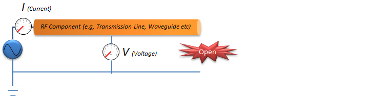
A source drives a line that is open at the far end. For a short time after switch on, the meters show a current even though the circuit is open.

• The source is the circle with a sine wave at the left, connected to ground at the bottom.
• The I (Current) meter sits between the source and the RF Component, labelled e.g. Transmission Line, Waveguide etc.
• The V (Voltage) meter is connected between the line and the ground return below it.
• The red star marks the far end of the line as Open.

Applying the concept described above, you would see the current and voltage for loger and longer as you use longer and longer RF Component because it takes longer time for the current from the source to reach the end of the circuit.

If we assume that we can extend the length of the RF component to inifinite length, the current would flow forever even though the circuit is open at the end because it would take forever for the current from the source to reach the end of the circuit. In this case, the current would flow in only one direction from the source to the end of the RF component because there would be no reflection from the end of the component. Assuming that the reflection happens only at the end of the component, there would be no chance for the signal get reflected because it would take infinate time (meaning never happens) to reach the end of the component.

Let's put numbers on the time scale. In a coaxial cable with a polyethylene dielectric, the relative permittivity is about 2.25, so the wave travels at c/1.5, about 2 x 10⁸ m/s. It needs 5 ns to travel 1 m. So on a 1 m cable, the source sees the incident wave alone for 10 ns, until the reflection from the open end returns. On a 10 m cable this time is 100 ns. The picosecond scale mentioned above fits a line of a few millimeters on a circuit board.

If you measure the current and voltage in this kind of ideal condition, you can calculate the impedance as follows.

Z = V/I

The Z (impendence) measured in this kind of ideal condition is called 'Characteristic Impedence' because the measured value is determined by 'physical/electrical characteristics of the RF component (e.g, material, physical dimension, shape etc).

For example, take a 1 V step source with a 50 ohm internal resistance, driving a 50 ohm line. During those first nanoseconds the line looks like a 50 ohm resistor. So the voltage meter reads 0.5 V, the current meter reads 10 mA, and V/I is 50 ohm, even though the far end is open.

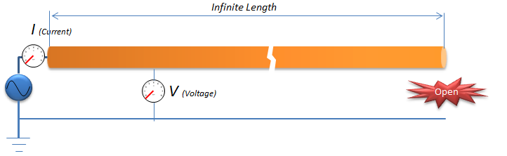
The same setup with a line of infinite length. The wave never reaches the open end, so no reflection ever comes back and the meters keep reading the ratio Z₀.

• The arrow above the line is labelled Infinite Length. The break in the middle of the line shows that part of the length is not drawn.
• The meters and the source are the same as in the open line picture above, and the Open mark sits at the far end.

Of course, you cannot build this kind of ideal circuit because you cannot make any RF component with infinite length.

• The source sees Z₀ before the reflection returns : for the round trip time of the line, the far end has no effect on the meters.
• The time scale depends on the length : a 1 m coaxial cable gives 10 ns before the reflection returns, and a board trace of a few millimeters gives picoseconds.
• An infinite line never reflects : so for an infinite line the input reading V/I equals Z₀ forever.

Which load makes a finite line look infinite ?

So let's think of more practical approach. Let's suppose you have a circuit as shown below. In this circuit, the circuit is not open, now it is a closed circuit and it is closed by a load labeled as Z_L (load impedance).

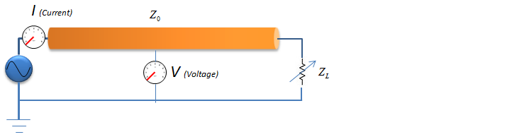
The practical circuit. A variable load Z_L closes the far end of a line of characteristic impedance Z₀.

• The line is labelled Z₀, and the source, the I (Current) meter and the V (Voltage) meter are the same as before.
• A resistor with an arrow across it, labelled Z_L, connects the far end of the line to the ground return. The arrow marks it as adjustable.

Assume that you just put any arbitrary value for the load impedance and you will see a certain value at Ampere meter and Voltimeter. However, in most case the value you read in the meter would not be same as the one you would see in the ideal case that I described above because some portions of the signal (source power) would get reflected at the end of the RF component.

With a lot of trials and a lot of luck (?), you may find a specific Z_L value at which you see the same Ampere meter value and Votimeter value as in the ideal case described above, the specific Z_L value at this condition become same as the characteristic impedance of the component. It means that the Z_L (Load Impedance) create the same effect of lengthening the RF component to the ininite length. (This is the meaning of the first definition at the beginning of this page)

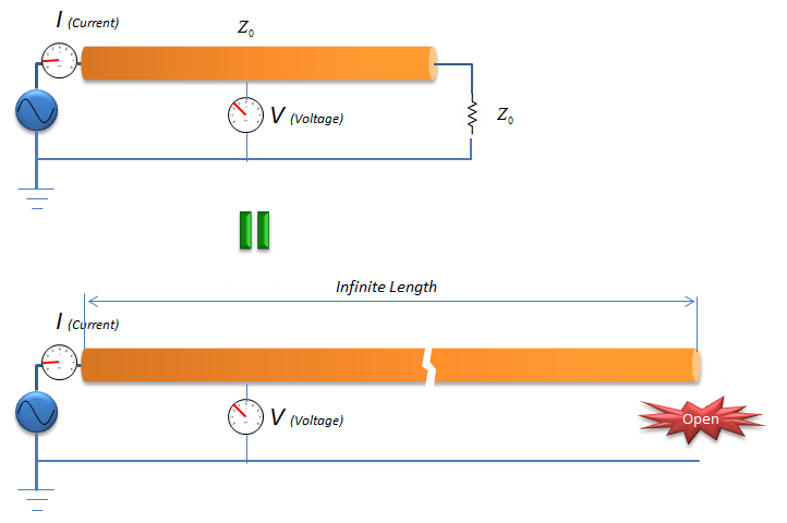
A line terminated in its own Z₀ gives the same meter readings as an infinitely long line.

• Top: the line Z₀ ends in a resistor labelled Z₀.
• Middle: a green equals sign.
• Bottom: the infinite length line with the Open mark, the same as in the infinite line picture above.

Now go back to the beginning of this page and read the sample definition of Characteristic Impedance and see if it make sense to you. If it does not make clear sense to you yet, read some other materials as listed below and try whatever you can search from google or other text book.

You do not need luck to find that load. The reflection coefficient at the load is Γ = (Z_L - Z₀)/(Z_L + Z₀). It is zero only when Z_L = Z₀, so the matching load is simply the characteristic impedance. The table below shows a few loads on a 50 ohm line. The return loss is -20 x log₁₀|Γ|, and the VSWR is (1 + |Γ|)/(1 - |Γ|).

Look at the 100 ohm and 25 ohm rows. A load twice Z₀ and a load half of Z₀ reflect the same power. Only the sign of Γ differs. The open line from the earlier section is the +1 row. That is why its meters change after the round trip time: the full wave comes back and adds to the incident one.

• The matched load is Z₀ itself : with Z_L = Z₀, the reflection coefficient is zero and the line looks infinitely long.
• Mismatch is measured by the reflection coefficient : Γ, return loss and VSWR are three ways of writing the same mismatch.
• An open and a short both reflect everything : they differ only in the sign of the reflected voltage.

What sets the value of the characteristic impedance ?

So far Z₀ has been a number that the meters read. The last question is where that number comes from, and why it depends on the shape and the material of the line rather than on its length.

A transmission line can be modelled as a chain of very short sections. Each section has a series resistance R and inductance L, and a shunt conductance G and capacitance C, all given per meter. For this model the characteristic impedance is Z₀ = √((R + jωL)/(G + jωC)). At RF, ωL is usually much larger than R and ωC much larger than G. Then the formula reduces to the lossless form Z₀ = √(L/C), which does not depend on frequency.

For example, a 50 ohm coaxial cable with a polyethylene dielectric has about L = 250 nH/m and C = 100 pF/m. Then √(L/C) = √2500 = 50 ohm. The same two numbers also give the wave speed 1/√(LC) = 2 x 10⁸ m/s, which matches the 5 ns per meter used in the open line example. L and C are set by the conductor sizes, their spacing and the dielectric, and the length never appears. The Coax page derives L, C and Z₀ from the dimensions of a coaxial cable.

• Z₀ comes from L and C per meter : for a low loss line, Z₀ = √(L/C), so it depends on geometry and material but not on length.
• The same L and C give the speed : the wave speed is 1/√(LC), so a line with a fixed Z₀ can still be fast or slow.
• Losses make Z₀ complex : at low frequency, where R and G are no longer small, the full formula applies and Z₀ changes with frequency.

Further Reading

The links below give other versions of the same explanation. Each one starts from a different definition, so reading two of them side by side helps you connect the definitions to the thought experiment above.

• What is Characteristic Impedance ?
• Characteristic Impedance
• Characteristic Impedance (Wikipedia)