IP3

As you learned from Amplifier page, most of the amplifier shows some unwanted nonlinear properties represented as the second order and third order or higher oder polynomial terms.

IP3, the third order intercept point, is the single number that tells you how strong the third order distortion of an amplifier or a mixer is. Let's first find the point on a simple polynomial. Then we will see how engineers measure it with two tones, how it relates to the 1 dB compression point, and how it adds up in a receiver chain. The Amplifier page covers the polynomial model itself.

Where does the IP3 point come from ?

Let's assume that we have an amplifier with third order polynomial. When a signal (e.g, sin wave) comes into the amplifier, the amplifier produces not only the linearly amplified signal but also the nonlinear components as well. What we want to do is to analyze the degree of those non-linear portions of the amplifier. The analysis is very simple.. it can be explained by high school math as shown below.

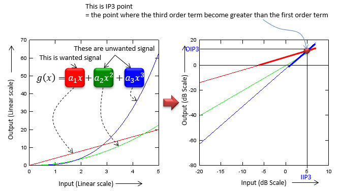
Linear, second order and third order terms of g(x) on a linear scale and on a dB scale, with the IP3 point marked

Figure 1. The three terms of g(x) = a₁x + a₂x² + a₃x³ on a linear scale and on a dB scale. On the dB scale each term is a straight line, and IP3 is where the third order line meets the first order line.

Let's look at the graph to the left first. You would see three graphs, the red one is generated by the first order term (linear amplification), the green one is generated by the second order term and the blue one is generated by the third order term.

As you see in the graph, when the input value (horizontal axis) is small, the value of the linear term(1st term, red graph) is greater than any other non linear term (blue or green), but as the input value gets larger and larger, you would notice that the blue (the third order term) and green (the second order) term gets larger at much higher rate than the red graph.. and eventually the blue and green gets larger than the red one. The point where the blue (the third order term) gets equal to the red (the first order term) is called Third Order Intercept point or IP3. This is very simple mathematical concept. But you wouldn't have seen this kind of graph (the graph on the left side) in your Rf/Amplifier text book. If you just change the scale of both x axis and y axis of the left graph, you would have the graph as shown on the right side. This would be the one you would have seen in the text book. The interpretation of the graph on the right side is exactly same as I expalined above. The reason why they convert the left side graph into the right side graph is that 'straight' line would be easier to understand and the slope of the each of the straight line can easily represent the degree of the effect created by the nonlinear terms.

Generally speaking, the higher IP3 value, the wider linear region that the amplifier has.

We can read the coefficients from the left graph and check the crossing point. The red line reaches 20 at x = 5, so a₁ = 4. The blue curve reaches about 62 at x = 5, so a₃ is about 0.5. The two terms are equal when a₃x³ = a₁x, which gives x = √(a₁/a₃) = 2.83 and an output of 11.3. The right graph takes 10 log₁₀ of these values, so the crossing moves to about 4.5 dB input and 10.5 dB output. This matches the IP3 marker near 5 dB in Figure 1.

The slopes on the right graph come straight from the powers of x. Taking the log turns xⁿ into n times log x. So the first order line has slope 1, the second order line has slope 2, and the third order line has slope 3. Every 1 dB of extra input adds 1 dB to the wanted output and 3 dB to the third order output.

Two cautions apply to Figure 1. First, a real amplifier never reaches its IP3. It compresses well before that point, so IP3 is found by extending the straight lines from low input levels. Second, the picture uses a positive a₃ to keep all curves above zero. A compressing amplifier has an a₃ with the opposite sign to a₁, but the intercept is defined by the size of the terms, so the idea is the same.

IP3 is where the third order line meets the linear line : on a dB scale the lines have slopes 1 and 3.
IP3 is an extrapolated point : the amplifier compresses long before its output reaches IP3.
A higher IP3 means a wider linear region : the third order term stays small up to a higher input level.

How is IP3 measured with two tones ?

A single sine wave into the cubic term creates a product at three times its frequency. That product is far outside the band, and a filter removes it easily. So a single tone hides the distortion that matters most. Two tones close to each other show it, because they create third order products right next to the wanted signals.

Suppose the input is A cos(2πf₁t) + A cos(2πf₂t). Expanding a₃x³ gives terms at 2f₁ - f₂ and 2f₂ - f₁, each with amplitude (3/4)a₃A³. The wanted output at f₁ and f₂ has amplitude a₁A for small A. For tones at 1000 MHz and 1001 MHz, the third order products fall at 999 MHz and 1002 MHz. These are the intermodulation products IM3, and Figure 2 shows where they sit.

Figure 2. Output spectrum of a two-tone test. The IM3 products sit one tone spacing outside each tone, so a band filter cannot remove them. ΔIM is the gap between a tone and its IM3 product.

Because the tones grow with slope 1 and the IM3 products grow with slope 3, the gap ΔIM shrinks by 2 dB for every 1 dB of extra input. The lines meet when ΔIM reaches 0. This gives the formula used on every test bench:

OIP3 = P_out + ΔIM/2 : P_out is the output power of one tone in dBm, and ΔIM is the tone to IM3 gap in dB.
IIP3 = OIP3 - G : G is the small signal gain in dB. You can also use P_in + ΔIM/2.

Let's work one example. Two tones of -20 dBm each go into an amplifier with 15 dB of gain. Each tone comes out at -5 dBm, and the IM3 products come out at -65 dBm. So ΔIM = 60 dB. Then OIP3 = -5 + 30 = 25 dBm, and IIP3 = 25 - 15 = 10 dBm. If you raise each input tone by 1 dB, the IM3 products rise by 3 dB, ΔIM drops to 58 dB, and the formula still gives the same IP3.

Two tones show the in-band distortion : the IM3 products at 2f₁ - f₂ and 2f₂ - f₁ sit next to the wanted signals.
ΔIM shrinks 2 dB per 1 dB of input : this is why the formula divides ΔIM by 2.
Measure at a low enough level : the formula holds only while IM3 still grows with slope 3. Near compression the result is no longer valid.

How does IP3 relate to the 1 dB compression point ?

Datasheets usually give both IP3 and P1dB, and the two numbers are related. Both come from the same third order term, so for a simple cubic model one number predicts the other. Knowing the relation helps you check whether a datasheet is consistent.

With a single tone of amplitude A, the cubic term adds (3/4)a₃A³ at the fundamental frequency. For a compressing amplifier this term subtracts from a₁A. The gain falls by 1 dB when (3/4)|a₃/a₁|A² = 1 - 10^-1/20 = 0.109. The input IP3 is at A² = (4/3)|a₁/a₃|. The ratio of the two powers is 9.6 dB. So for this model the input P1dB is about 9.6 dB below IIP3.

Real devices do not follow the cubic model exactly. Fifth order and higher terms also affect compression, so the measured gap is often different from 9.6 dB. Use the relation as a check, not as a replacement for measuring both. See 1dB Compression Point for the compression side.

IP3 also sets the spurious free dynamic range, SFDR. This is the range of input levels over which the IM3 products stay below the noise floor. In dB it is SFDR = (2/3) x (IIP3 - N), where N is the input-referred noise floor in dBm. For IIP3 = 10 dBm and N = -100 dBm, SFDR = (2/3) x 110 = 73.3 dB. See Dynamic Range.

For a cubic model, P1dB is 9.6 dB below IIP3 : both points come from the same a₃/a₁ ratio.
Real devices differ : higher order terms change compression, so treat the 9.6 dB as a consistency check.
IP3 sets the spurious free dynamic range : SFDR = (2/3) x (IIP3 - N) in dB.

How does IP3 add up in a receiver chain ?

A receiver is a chain of an LNA, a mixer and more stages, and we need the IP3 of the whole chain. The answer is the mirror image of the noise figure problem. For noise, the first stage matters most. For IP3, the last stages usually matter most, because they see the signal after all the gain in front of them.

The input IP3 of a cascade follows 1/IIP3_total = 1/IIP3₁ + G₁/IIP3₂ + G₁G₂/IIP3₃ + ... Here every IIP3 is in mW and every gain is a linear ratio, not dB. The formula assumes that the IM3 products of the stages add in phase, which is the worst case.

Let's take an LNA with 15 dB of gain and an IIP3 of 0 dBm, followed by a mixer with an IIP3 of +10 dBm. In linear terms, 1/1 + 31.6/10 = 4.16, so IIP3_total = 0.24 mW = -6.2 dBm. The mixer is 10 dB better than the LNA on paper, but the 15 dB of LNA gain in front of it makes it the weaker stage. More LNA gain would lower the noise figure and lower the IIP3 even more. This is the basic trade-off in receiver planning.

Later stages limit the cascade IP3 : each stage is divided by the total gain in front of it.
Gain helps noise figure and hurts IP3 : receiver planning balances the two. See Noise Figure.
Work in linear units : convert IIP3 to mW and gain to a ratio before adding, then convert back to dBm.