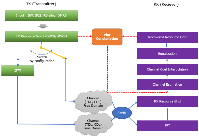
For this note, is a comprehensive Python script for simulating 5G NR PDSCH (Physical Downlink Shared Channel) transmission through various radio channel models. The tool implements both frequency-domain and time-domain channel processing, supports multiple channel models (AWGN, TDL, CDL), and provides channel estimation, equalization, and BER analysis capabilities...

Followings are brief descriptions on each procedure with the focus on sionna api

• Inputs: Channel bandwidth, subcarrier spacing, RB allocation, channel type (AWGN/TDL/CDL), SNR, channel estimation/equalization methods, DMRS configuration
• Resource Grid Generation: Creates OFDM resource grid with DMRS and CORESET support
  • Sionna API: ResourceGrid, ResourceGridMapper, PilotPattern
• Data Symbol Generation: Generates random bits and maps to constellation symbols (16QAM)
  • Sionna API: BinarySource, Mapper
• Channel Processing (selectable via use_time_domain_channel option):
  • Frequency Domain (default): TX Resource Grid → Channel (Freq Domain) → AWGN → RX Resource Grid (direct frequency-domain multiplication, no OFDM mod/demod)
    • Custom implementation (NumPy-based channel coefficient generation)
    • Optional: Sionna TDL/CDL models if available (falls back to custom)
  • Time Domain: TX Resource Grid → IFFT → Channel (Time Domain) → AWGN → FFT → RX Resource Grid (full OFDM modulation/demodulation with time-domain channel convolution)
    • Custom implementation (NumPy IFFT/FFT, custom channel IR generation)
    • Optional: Sionna TDL/CDL models if available (falls back to custom)
• Channel Estimation: LS (Least Squares) or MMSE (Minimum Mean Square Error) estimation on DMRS REs extracted from TX and RX resource grids
  • Custom implementation (NumPy-based LS/MMSE algorithms)
• Channel Coefficient Interpolation: Interpolates channel estimates from DMRS REs across frequency and time to cover all resource elements
  • Sionna API: LinearInterpolator (if available, otherwise custom cubic spline interpolation)
• Equalization: ZF (Zero Forcing) or MMSE equalization using interpolated channel coefficients
  • Custom implementation (NumPy-based ZF/MMSE algorithms)
• BER Analysis: Bit Error Rate calculation with constellation visualization comparing TX and recovered symbols
  • Custom implementation (constellation matching and bit error counting)
• Visualization: Interactive Tkinter GUI with multiple tabs showing resource grids, channel coefficients, constellations, and spectrum
  • Custom implementation (Tkinter/Matplotlib-based GUI)

Toolkits for the script

I didn't write the code myself. What I did was just prompting for AI tool and did basic check up for the output. Followings are the tool kits that I used for this script

• Scripting IDE : Cursor
• Version: 2.1.50 (system setup)
• VSCode Version: 1.105.1
• Commit: 56f0a83df8e9eb48585fcc4858a9440db4cc7770
• Date: 2025-12-06T23:39:52.834Z
• Electron: 37.7.0
• Chromium: 138.0.7204.251
• Node.js: 22.20.0
• V8: 13.8.258.32-electron.0
• OS: Windows_NT x64 10.0.26100
• AI Model : Auto (as of Dec 11, 2025)
• Python Info : Check out this note for the detailed installation proces that I went through

==== Python Version ==== 3.12.3 (main, Nov  6 2025, 13:44:16) [GCC 13.3.0]   ==== Python Executable ==== /home/jaeku/nvidia/venv-sionna/bin/python3   ==== Platform Info ==== Linux-6.6.87.2-microsoft-standard-WSL2-x86_64-with-glibc2.39 ('main', 'Nov  6 2025 13:44:16')   ==== Site-Packages Directories ==== ['/home/jaeku/nvidia/venv-sionna/lib/python3.12/site-packages', '/home/jaeku/nvidia/venv-sionna/local/lib/python3.12/dist-packages', '/home/jaeku/nvidia/venv-sionna/lib/python3/dist-packages', '/home/jaeku/nvidia/venv-sionna/lib/python3.12/dist-packages']   ==== sys.path ====   /home/jaeku/nvidia   /usr/lib/python312.zip   /usr/lib/python3.12   /usr/lib/python3.12/lib-dynload   /home/jaeku/nvidia/venv-sionna/lib/python3.12/site-packages   ==== Installed Packages ==== absl-py == 2.3.1 asttokens == 3.0.1 astunparse == 1.6.3 certifi == 2025.11.12 charset-normalizer == 3.4.4 comm == 0.2.3 contourpy == 1.3.3 cycler == 0.12.1 decorator == 5.2.1 drjit == 1.2.0 executing == 2.2.1 flatbuffers == 25.9.23 fonttools == 4.61.0 gast == 0.7.0 google-pasta == 0.2.0 grpcio == 1.76.0 h5py == 3.15.1 idna == 3.11 importlib_resources == 6.5.2 ipydatawidgets == 4.3.5 ipython == 9.8.0 ipython_pygments_lexers == 1.1.1 ipywidgets == 8.1.8 jedi == 0.19.2 jupyterlab_widgets == 3.0.16 keras == 3.12.0 kiwisolver == 1.4.9 libclang == 18.1.1 Markdown == 3.10 markdown-it-py == 4.0.0 MarkupSafe == 3.0.3 matplotlib == 3.10.7 matplotlib-inline == 0.2.1 mdurl == 0.1.2 mitsuba == 3.7.1 ml_dtypes == 0.5.4 namex == 0.1.0 numpy == 1.26.4 opt_einsum == 3.4.0 optree == 0.18.0 packaging == 25.0 parso == 0.8.5 pexpect == 4.9.0 pillow == 12.0.0 pip == 25.3 prompt_toolkit == 3.0.52 protobuf == 6.33.2 ptyprocess == 0.7.0 pure_eval == 0.2.3 Pygments == 2.19.2 pyparsing == 3.2.5 python-dateutil == 2.9.0.post0 pythreejs == 2.4.2 requests == 2.32.5 rich == 14.2.0 scipy == 1.16.3 setuptools == 80.9.0 sionna == 1.2.1 sionna-rt == 1.2.1 six == 1.17.0 stack-data == 0.6.3 tensorboard == 2.20.0 tensorboard-data-server == 0.7.2 tensorflow == 2.20.0 termcolor == 3.2.0 traitlets == 5.14.3 traittypes == 0.2.3 typing_extensions == 4.15.0 urllib3 == 2.6.0 wcwidth == 0.2.14 Werkzeug == 3.1.4 wheel == 0.45.1 widgetsnbextension == 4.0.15 wrapt == 2.0.1

Source Code and Output

You can get the source code for this note here.  I would not describe / explain on every single line of the code since AI (e.g, chatGPT, Gemini etc) will explain better than I do.

Disclaimer !!!

I have checked and fixed some obvious issues of the script while I am prompting the script, but I haven't verified all the details of the implementation. So there likely to be bugs / errors that I missed.  So take this purely as an educational purpose for getting some high level idea on how 3GPP NR Phy specification can be implemented

The script output some part of the result in text and some part in graphics.

Followings are the output of the code in text

User Interface (GUI) Overview

Followings are the snapshots of graphical output (NOTE : If you want to get images for better resolution, I would suggest you to install the sionna on your PC and run the script that I shared).

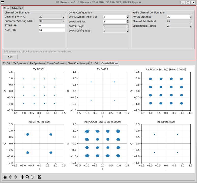
The GUI provides a compact, real-time view of the 5G NR PDSCH simulation flow from data generation from RX and final recover on RX side.

It is designed to expose the key configuration knobs and signal observation points without overwhelming the user with internal implementation details.

Basic Configuration Panels

The top section of the UI is dedicated to simulation configuration.It is split into three logical groups that mirror the structure of the link model.

Followings are brief descriptions of each part in this view :

• Channel Configuration panelcontrols the physical layout of the NR resource grid.
• Parameters such as channel bandwidth, subcarrier spacing, starting RB index, and number of allocated RBs define the frequency-domain structure of the OFDM grid.
• DMRS Configuration panelcontrols how reference signals are embedded into the grid.
• This includes the DMRS symbol index, additional positions, length, and configuration type.
• These parameters directly affect channel estimation accuracy and interpolation behavior.
• Radio Channel Configuration panel controls the impairments and receiver algorithms.
• AWGN SNR sets the noise level.
• Channel estimation and equalization methods determine how the receiver attempts to recover the transmitted symbols.
• Any change in these fields updates the simulation logic.
• Run regenerates the full transmit-channel-receive chain using the new settings.

Advanced Configuration Panels

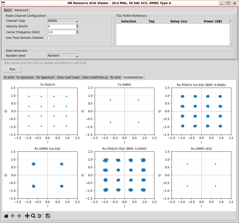
In Advanced configuration following following parameters are available. The Advanced configuration exposes parameters that affect channel dynamics, waveform realism, and repeatability. These options are not required for basic link validation, but they become important when studying time variation, Doppler effects, and channel selectivity.

Followings are brief descriptions of each part in this view :

• Radio Channel Configuration
• The Channel Type parameter selects the high-level channel model used in the simulation. It support three options : AWGN, TDL, TDL User and CDL
• AWGN represents a flat, non-fading channel and is mainly used for baseline verification.
• TDL and CDL enable multipath fading behavior and introduce frequency selectivity and time variation.
• The Velocity parameter controls Doppler effects.
• When set to zero, the channel remains time-invariant across OFDM symbols.
• A non-zero value introduces time variation in the channel coefficients, which directly impacts DMRS tracking and interpolation accuracy.
• The Carrier Frequency parameter defines the RF carrier used for Doppler calculations.
• It does not affect baseband sampling directly, but it determines how velocity translates into Doppler spread.
• Higher carrier frequency results in stronger Doppler effects for the same UE speed.
• The Use Time Domain Channel option selects the channel processing path.
• When disabled, the channel is applied directly in the frequency domain as a per-subcarrier complex gain.
• When enabled, the signal passes through full OFDM modulation, time-domain convolution with a channel impulse response, and OFDM demodulation.
• This switch allows direct comparison between simplified and physically accurate channel modeling.
• TDL Profile Reference
• The TDL Profile table becomes active only when TDL User is selected as the channel type.
• In this mode, the predefined 3GPP TDL profiles are not used. Instead, the channel impulse response is constructed directly from the entries in the table.
• Each row in the table represents one multipath tap.
• The delay and power values define the relative timing and strength of that path.
• The Selection field allows the user to enable or disable individual taps.
• Only the taps explicitly selected in the table are applied to the channel model.
• This mechanism allows the user to:
• isolate a single multipath component,
• construct a custom multipath profile,
• or incrementally add taps to observe their impact.
• Multiple taps can be selected simultaneously.
• In this case, the resulting channel is the superposition of all selected taps.
• This design provides fine-grained control over the channel model.
• It is particularly useful for debugging, educational experiments, and sensitivity analysis of channel estimation and equalization behavior.
• Data Generator Configuration
• The Random Seed parameter controls the reproducibility of the simulation.
• When set to a fixed value, the same bit sequence and noise realization are generated every run.
• This is useful for debugging, regression testing, and algorithm comparison.
• When random mode is selected, each run produces a new data sequence.
• This is useful for BER averaging and stress testing under varying conditions.

Visualization Tabs

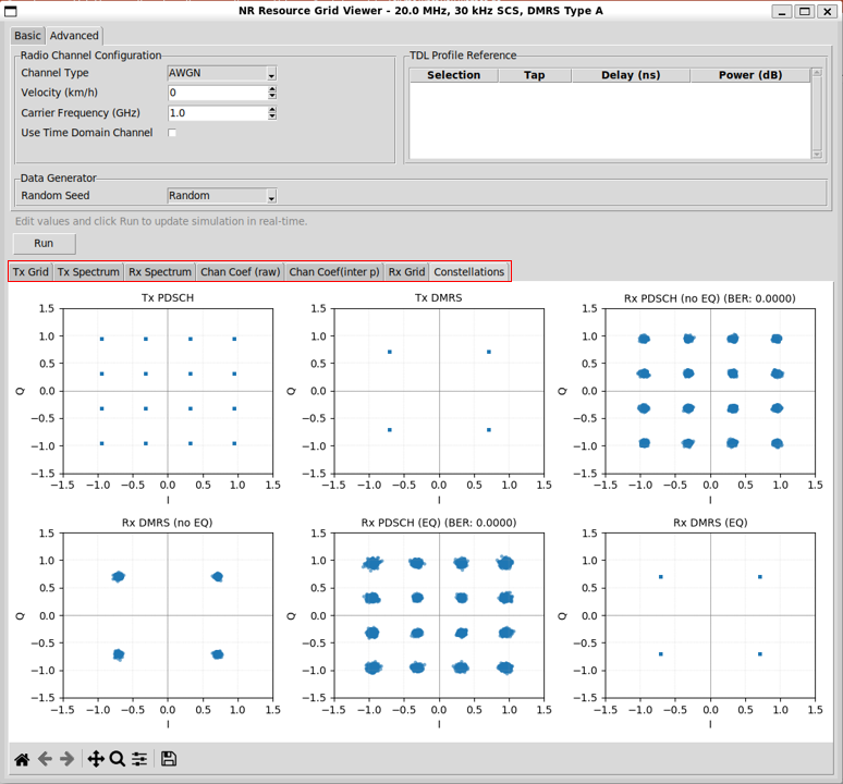
The Visualization tabs present the signal at key observation points along the end-to-end data path, starting from symbol generation at the transmitter and ending at symbol recovery at the receiver.

• Each tab corresponds to a specific processing stage.
• Together, they allow the user to follow how the signal evolves through modulation, channel distortion, estimation, and equalization.

Visualization Tab - Tx Grid

The Tx Grid panel visualizes the transmitted NR OFDM resource grid before any channel impairment is applied. It provides a direct view of how frequency–time resources are populated based on the current configuration.

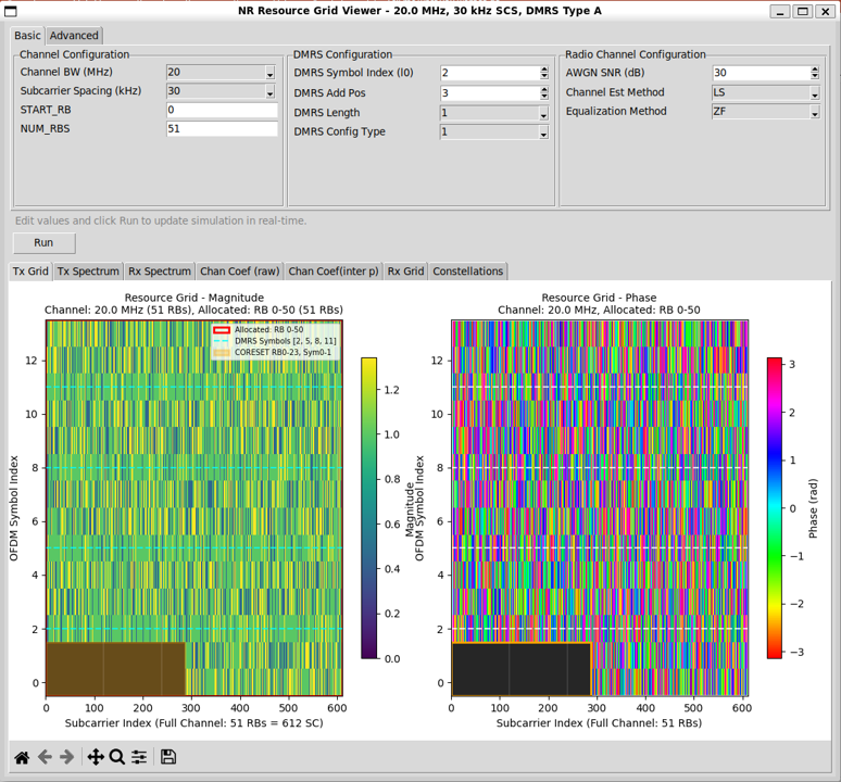
Followings are brief descriptions of each part in this view :

• Resource Grid Representation
• The left plot shows the magnitude of the transmitted resource grid.
• Each pixel represents one resource element.
• The horizontal axis corresponds to the subcarrier index across the full channel bandwidth.
• The vertical axis corresponds to the OFDM symbol index within the slot.
• Only the RBs specified by the allocation parameters are populated with data.
• Unallocated RBs appear as empty or masked regions.
• DMRS locations are overlaid and highlighted.
• This makes the reference signal structure immediately visible within the grid.
• Phase Visualization
• The right plot shows the phase of the transmitted resource grid.
• Phase is displayed in radians and mapped to color.
• This view is useful for:
• confirming symbol randomness,
• verifying constellation mapping,
• and identifying structured signals such as DMRS.
• Regions without transmitted symbols appear as blank or masked areas.

Visualization Tab - Tx Spectrum

The Tx Spectrum panel visualizes the spectral characteristics of the transmitted NR signal before it passes through the radio channel. It provides a frequency-domain view that complements the time–frequency view of the Tx Grid.

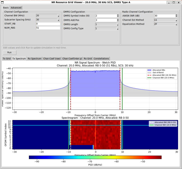
Followings are brief descriptions of each part in this view :

• Power Spectral Density View
• The upper plot shows the power spectral density (PSD) of the transmitted signal, computed using a Welch method.
• The horizontal axis represents frequency offset from the carrier.
• The vertical axis represents power spectral density.
• The shaded central region corresponds to the RBs allocated for transmission.
• Vertical markers indicate the boundaries of:
• allocated bandwidth,
• and the full channel bandwidth.
• This view allows verification that:
• the occupied bandwidth matches the RB allocation,
• the signal is correctly centered around the carrier,
• and out-of-band regions contain only noise or leakage.
• Spectrogram View
• The lower plot shows a spectrogram, displaying power distribution over frequency and OFDM symbol index.
• The horizontal axis again represents frequency offset.
• The vertical axis represents OFDM symbol index.
• Allocated RBs appear as a bright, continuous region across symbols.
• Unallocated regions appear dark.
• This view helps confirm:
• time consistency of transmission,
• absence of unintended spectral hopping,
• and alignment between frequency allocation and OFDM symbol structure.

Visualization Tab - Rx Spectrum

The Rx Spectrum panel visualizes the spectral characteristics of the received signal after it has passed through the configured radio channel. It allows direct comparison with the Tx Spectrum to observe how the channel and noise affect the signal in the frequency domain.

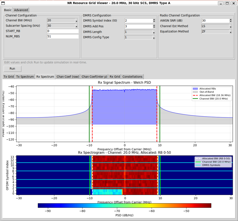
Followings are brief descriptions of each part in this view :

• Power Spectral Density View
• The upper plot shows the power spectral density (PSD) of the received signal, computed using the same Welch method as the transmitter view.
• The horizontal axis represents frequency offset from the carrier.
• The vertical axis represents power spectral density.
• The allocated RB region remains clearly visible, but the spectral floor is elevated due to noise.
• Depending on the channel configuration, additional spectral shaping or distortion may be visible.
• Vertical markers again indicate:
• allocated bandwidth,
• and full channel bandwidth.
• This view makes it easy to assess:
• effective SNR,
• out-of-band noise leakage,
• and overall spectral integrity after transmission.
• Spectrogram View
• The lower plot shows the received spectrogram, displaying power across frequency and OFDM symbol index.
• Compared to the Tx spectrogram, the received view shows:
• noise-induced power spread,
• possible frequency selectivity,
• and time variation if Doppler is enabled.
• DMRS symbol locations are overlaid.
• This helps correlate channel estimation performance with observed spectral behavior.

Visualization Tab - Channel Coefficient (Raw)

The Channel Coef (raw) panel visualizes the direct output of the channel estimation stage.It shows channel coefficients estimated only at DMRS resource elements, without any interpolation across time or frequency.

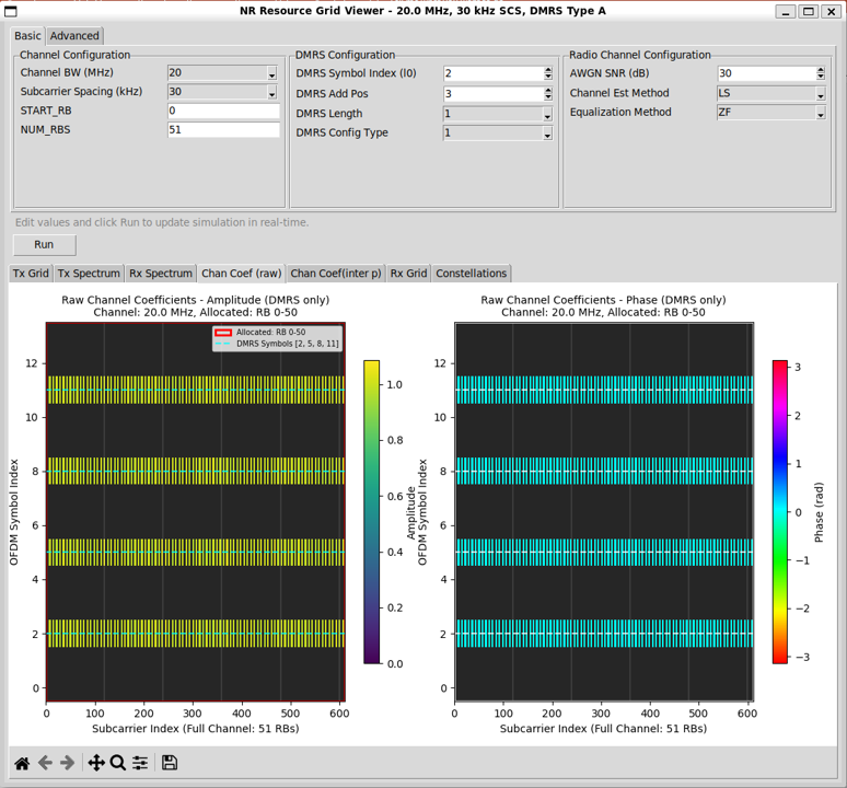
Followings are brief descriptions of each part in this view :

• Amplitude and Phase Views
• The left plot shows the amplitude of the estimated channel coefficients.
• The right plot shows the phase of the estimated channel coefficients.
• The horizontal axis represents the subcarrier index across the full channel bandwidth.
• The vertical axis represents the OFDM symbol index.
• Only OFDM symbols that contain DMRS are populated.
• Non-DMRS symbols appear empty, making the sparsity of reference signals explicit.
• Interpretation
• Each visible point corresponds to a channel estimate derived from a DMRS RE.
• No smoothing or averaging is applied beyond the estimator itself.
• This view reflects:
• the raw impact of noise,
• frequency selectivity of the channel,
• and any time variation present between DMRS symbols.
• In AWGN or flat fading cases, amplitude and phase appear relatively uniform.
• In multipath channels, frequency-dependent variation becomes visible.

Visualization Tab - Channel Coefficient (Inter p)

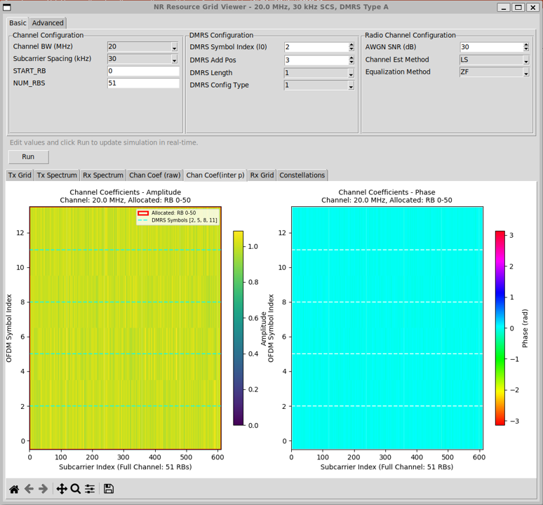
The Channel Coef (interp) panel visualizes the channel coefficients after interpolation across the full resource grid. It represents the channel knowledge actually used by the equalizer.

Followings are brief descriptions of each part in this view :

• Amplitude and Phase Views
• The left plot shows the interpolated channel amplitude.
• The right plot shows the interpolated channel phase.
• The horizontal axis represents the subcarrier index across the full channel bandwidth.
• The vertical axis represents the OFDM symbol index.
• Unlike the raw channel view, all OFDM symbols and all allocated subcarriers are populated.
• This reflects the expansion of sparse DMRS-based estimates into a full-grid channel model.
• Interpolation Effect
• Interpolation fills in channel values between DMRS symbols in both time and frequency.
• In flat or slowly varying channels, the interpolated amplitude and phase appear smooth and uniform.
• In frequency-selective or time-varying channels, gradual transitions become visible.
• The dashed horizontal lines indicate DMRS symbol locations.
• These lines show the anchor points from which interpolation is performed.
• Why Channel Interpolation Is Needed
• In an ideal world, the receiver would know the channel coefficient for every resource element (RE) that carries PDSCH data.
• In reality, the receiver does not observe the channel everywhere.
• What the Receiver Actually Knows
• The channel can only be directly estimated on known symbols.
• In NR PDSCH, those known symbols are DMRS.
• For each DMRS RE, the receiver can compute the channel as:
• Received DMRS ÷ Transmitted DMRS → Channel estimate
• This gives channel coefficients only at DMRS locations.
• All other REs carry unknown data symbols, so the channel cannot be directly measured there.
• The Gap Between DMRS and PDSCH
• PDSCH occupies many more REs than DMRS.
• DMRS is intentionally sparse in both time and frequency to reduce overhead.
• As a result:
• channel estimates exist only at a small subset of REs,
• but equalization requires a channel coefficient at every PDSCH RE.
• This mismatch is the fundamental reason interpolation is required.
• What Interpolation Does
• Channel interpolation fills in the missing channel coefficients between DMRS positions.
• It uses the assumption that:
• the channel varies smoothly in frequency (limited delay spread),
• and slowly in time (limited Doppler).
• Using these assumptions, interpolation estimates the channel at data REs by:
• interpolating across subcarriers,
• interpolating across OFDM symbols,
• or both.
• The result is a full-grid channel estimate aligned with the PDSCH REs.
• Why Equalization Depends on Interpolation
• Equalization compensates the received symbol as:
• Received symbol ÷ Channel coefficient → Equalized symbol
• This operation must be done per RE.
• Without interpolation:
• the equalizer only knows the channel at DMRS REs,
• PDSCH REs would have no channel reference,
• equalization would be impossible.
• So interpolation is not an optimization.
• It is a structural requirement.

Visualization Tab - Rx Grid

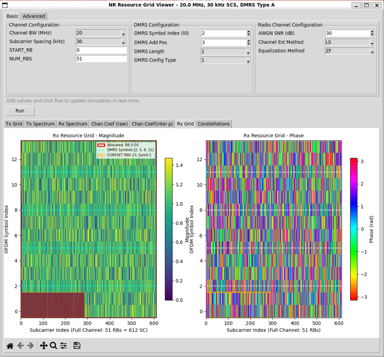
The Rx Grid panel visualizes the received OFDM resource grid after channel equalization. It represents the frequency–time signal that is passed to symbol decision and demapping.

Followings are brief descriptions of each part in this view :

• Resource Grid Representation
• The left plot shows the magnitude of the equalized resource grid.
• The right plot shows the phase of the equalized resource grid.
• The horizontal axis represents the subcarrier index across the full channel bandwidth.
• The vertical axis represents the OFDM symbol index.
• Allocated RBs are populated with equalized symbols.
• Unallocated regions remain masked.
• DMRS symbol locations are overlaid for reference, even though they are not used for data detection.
• Interpretation
• After equalization, the channel effects should be largely removed.
• In ideal conditions, the magnitude becomes uniform across REs.
• The phase becomes randomly distributed according to the transmitted constellation rather than the channel response.
• Any residual distortion visible here originates from:
• channel estimation error,
• interpolation error,
• noise enhancement during equalization.

Visualization Tab - Constellation

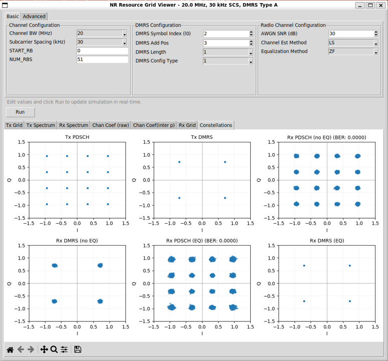
The Constellations view provides a symbol-level summary of the entire transmission and reception process. It condenses all preceding processing stages into a small set of intuitive plots that directly reflect system performance.

Followings are brief descriptions of each part in this view :

• Transmitter Reference Constellations
• The Tx PDSCH plot shows the ideal transmitted data constellation.
• It serves as the reference for evaluating distortion and recovery.
• The Tx DMRS plot shows the transmitted reference symbols.
• These points are fixed and known to the receiver.
• Receiver Constellations Before Equalization
• The Rx PDSCH (no EQ) plot shows received data symbols before equalization.
• Channel distortion and noise are clearly visible as spreading and rotation of constellation points.
• The Rx DMRS (no EQ) plot shows received DMRS symbols before equalization.
• These points form the basis for channel estimation.
• Receiver Constellations After Equalization
• The Rx PDSCH (EQ) plot shows recovered data symbols after channel estimation, interpolation, and equalization.
• The Bit Error Rate (BER) is displayed alongside this plot.
• The Rx DMRS (EQ) plot shows equalized DMRS symbols.
• These points should collapse back to their original reference locations if equalization is effective.
• Interpretation
• A tight clustering of equalized PDSCH symbols around ideal constellation points indicates good channel estimation and equalization.
• Residual spreading reflects:
• noise,
• interpolation error,
• and channel estimation inaccuracies.
• BER provides a quantitative metric that complements the visual inspection.

Advanced Test - TDL

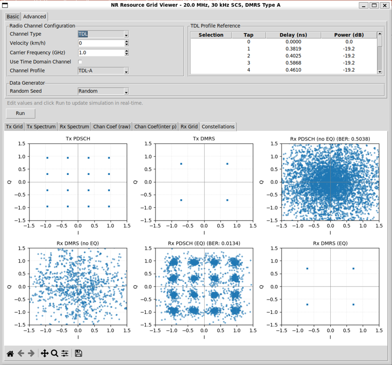
This example demonstrates the effect of a multipath fading channel using a TDL model. The test is executed by selecting TDL as the channel type in the Advanced configuration and pressing Run.

Followings are brief descriptions of each part in this view :

• Test Setup
• The channel type is set to TDL.
• A predefined TDL-A profile is selected.
• The velocity is set to zero, so the channel is time-invariant but frequency-selective.
• AWGN is still present according to the configured SNR.
• Observations in Constellation View
• Before equalization, the Rx PDSCH (no EQ) constellation is heavily smeared.
• The symbols form a near-continuous cloud, and the BER is close to random decision levels.
• The Rx DMRS (no EQ) constellation shows similar distortion.
• These distorted DMRS symbols are used for channel estimation.
• After channel estimation, interpolation, and equalization, the Rx PDSCH (EQ) constellation collapses back toward the ideal constellation points.
• The BER drops significantly compared to the no-equalization case.
• The Rx DMRS (EQ) constellation aligns closely with the transmitted reference points.
• This confirms that the estimated channel effectively compensates the multipath distortion.
• Interpretation
• This example highlights the role of the receiver processing chain.
• Multipath fading severely distorts the signal when left uncompensated.
• Channel estimation and interpolation reconstruct the frequency-selective channel.
• Equalization removes most of the distortion on a per-RE basis.
• Residual spreading and non-zero BER reflect:
• noise,
• interpolation error,
• and limited DMRS density.

Advanced Test - User TDL

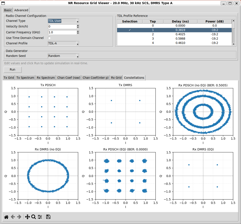
This example demonstrates the User TDL mode, where the multipath channel is constructed only from explicitly selected taps in the TDL Profile table. (NOTE : When User TDL is selected, 'Use Time Domain Channel' is automatically unchecked since this is designed to be applied only to frequency domain resource grid) The test is executed by selecting TDL User as the channel type and pressing Run.

Followings are brief descriptions of each part in this view :

• User TDL Mode Behavior
• In TDL User mode, predefined TDL profiles are not applied as a whole.
• Instead, the channel impulse response is built only from the taps selected in the TDL Profile table.
• Each row in the table represents one multipath tap with a specific delay and power.
• A tap can be enabled or disabled by double-clicking the row.
• Only rows marked as selected contribute to the channel.
• Unselected taps are completely ignored.
• Multiple taps can be selected at the same time.
• The resulting channel is the superposition of all selected taps.
• Observation from the Example
• In this example, only a subset of taps is selected.
• Before equalization, the Rx PDSCH (no EQ) constellation forms structured rings rather than a random cloud.
• This pattern reflects deterministic phase rotation caused by a small number of discrete delay components.
• The Rx DMRS (no EQ) constellation shows the same circular distortion.
• These distorted reference symbols are used for channel estimation.
• After channel estimation, interpolation, and equalization, the Rx PDSCH (EQ) constellation collapses back to the ideal constellation points.
• The BER drops to zero in this example.
• The Rx DMRS (EQ) constellation aligns with the transmitted DMRS points, confirming correct channel compensation.
• Why This Mode Is Useful
• User TDL mode allows precise control over channel structure.
• It is useful for:
• isolating the effect of a single multipath component,
• studying phase rotation caused by fixed delays,
• validating channel estimation and equalization logic,
• and teaching the relationship between impulse response and constellation distortion.
• Compared to predefined TDL profiles, this mode makes the channel behavior predictable and explainable, which is ideal for debugging and educational experiments.

Advanced Test - User CDL

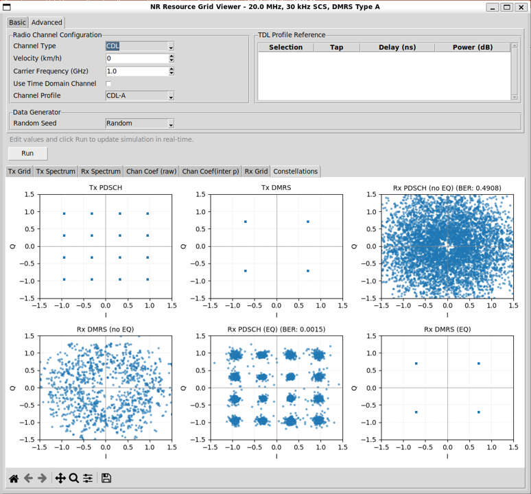
This example demonstrates the use of a CDL (Clustered Delay Line) channel model. The test is executed by selecting CDL as the channel type in the Advanced configuration and pressing Run.

Followings are brief descriptions of each part in this view :

• CDL Channel Characteristics
• The CDL model represents a more realistic propagation environment than TDL.
• Instead of independent taps, the channel is composed of clusters, each containing multiple rays with:
• different delays,
• different powers,
• and different phases.
• Even when velocity is set to zero, the superposition of many rays produces strong frequency selectivity.
• Compared to TDL, CDL introduces:
• richer multipath structure,
• stronger amplitude variation,
• and more complex phase behavior.
• Observations in Constellation View
• Before equalization, the Rx PDSCH (no EQ) constellation is heavily distorted.
• The symbols spread into a dense cloud, and the BER is close to random decision levels.
• The Rx DMRS (no EQ) constellation shows similar dispersion.
• These noisy and distorted DMRS symbols are used for channel estimation.
• After channel estimation, interpolation, and equalization, the Rx PDSCH (EQ) constellation converges back toward the ideal constellation points.
• The BER drops dramatically, though it may not reach zero due to residual estimation and interpolation errors.
• The Rx DMRS (EQ) constellation aligns closely with the transmitted DMRS points, indicating effective channel compensation.

Source Code Overview

Even though I no longer need to describe every single line of code in the age of AI, I still think it is valuable to write down some key points. This is not to show off the code itself. It is to record the intention behind the script. I want to clarify what I was trying to do, what kind of idea I had in mind, and what kind of problems this script is designed to solve. This allows the reader to connect the final result with the original design goal. It also helps me later when I come back to this code after a long time and forget my own thinking process.

You may not need all of these details if your only goal is to understand the output of the script. For simple usage, you can often treat the script as a black box. You run it. You look at the result. You move on. In many cases this is enough. However, if you want to modify, revise, or extend the script for your own purpose, the situation changes. You would need to know which part of the code is doing what. You would need to know which parameters control which behavior. You would also need to know what kind of assumptions I made when I first wrote the code. In that case, a clear description of the code is not a luxury. It becomes a kind of map.

One of the best ways to learn anything related to programming is still very old-fashioned. You break it and then you fix it. You change a small part of the script and see what goes wrong. You check the error. You adjust. You run it again. This loop may look inefficient at first, but it forces your brain to connect cause and effect inside the code. So my intention with these explanations is not just to document the script. It is to give you enough context so that you can safely break it, understand why it broke, and then fix it in a way that matches your own idea. This process is painful sometimes, but it is also the part that makes the knowledge stick to your brain.

Key Features

• Dual Channel Processing Modes: Frequency-domain (fast) and time-domain (realistic) channel application
• Multiple Channel Models: AWGN, TDL (Tapped Delay Line), and CDL (Clustered Delay Line) with various profiles
• Channel Estimation: LS and MMSE methods with frequency/time interpolation
• Equalization: ZF and MMSE equalizers
• Doppler Support: Time-varying channels with velocity-based Doppler shift
• 3GPP-Compliant DMRS: DMRS Type A with configurable positions, CDM groups, and OCC
• CORESET Support: Configurable CORESET regions with bitmap-based allocation
• Interactive GUI: Real-time configuration and visualization with tabbed interface
• BER Analysis: Comprehensive BER calculation and constellation visualization

Fully Implemented

Partially Implemented

Not Implemented

Description of Parameters (Global Variables)

Channel Bandwidth Configuration

Antenna Configuration

Channel Configuration

Channel Estimation and Equalization

DMRS Configuration

Data Generator Configuration

Description of Functions

Main Simulation Function

Runs the complete NR PDSCH simulation pipeline.

Parameters:

Returns: SimResult - Dataclass containing:

• x_rg: Transmitted resource grid tensor
• dmrs_mask_original: Original DMRS mask
• reserved_mask: Reserved RE mask
• rx_grid_no_eq: Received grid before equalization
• rx_grid_eq: Received grid after equalization
• constellations: Dictionary of constellation data for visualization
• ber_pdsch_no_eq: BER without equalization
• ber_pdsch_eq: BER with equalization
• h_est_full: Full channel estimate (interpolated)
• h_est_dmrs: Raw channel estimate at DMRS positions only
• Derived parameters (fft_size, num_subcarriers, etc.)

Processing Steps:

1. Compute derived parameters (FFT size, guard carriers, etc.)
2. Create DMRS pilot pattern
3. Create resource grid and mapper
4. Generate and map data symbols (16QAM)
5. Apply channel (frequency or time domain based on use_time_domain_channel)
6. Channel estimation on DMRS REs
7. Channel interpolation across all REs
8. Equalization (ZF or MMSE)
9. BER calculation
10. Return results for visualization

Channel Estimation Functions

Least Squares (LS) channel estimation.

Parameters:

Returns: np.ndarray - Channel estimates: rx_pilots / tx_pilots

Minimum Mean Square Error (MMSE) channel estimation.

Parameters:

Returns: np.ndarray - MMSE channel estimates

Algorithm:

• First computes LS estimate: h_ls = rx_pilots / tx_pilots
• Applies MMSE smoothing: h_mmse = h_ls * (snr / (snr + 1))

Interpolates channel estimates across frequency (within DMRS symbols) and time (copy nearest DMRS symbol for data symbols).

Parameters:

Returns: np.ndarray - Interpolated channel estimate covering all REs

Algorithm:

1. Uses Sionna LinearInterpolator if available, otherwise falls back to custom implementation
2. For each DMRS symbol: interpolates across frequency using cubic spline (magnitude and phase separately)
3. For data symbols: copies channel from nearest DMRS symbol in time

Equalization Functions

Zero Forcing (ZF) equalization.

Parameters:

Returns: np.ndarray - Equalized signal: rx_signal / h_est

Minimum Mean Square Error (MMSE) equalization.

Parameters:

Returns: np.ndarray - MMSE equalized signal

Algorithm:

• MMSE equalizer: h_mmse = conj(h_est) / (|h_est|^2 + 1/snr)
• Equalized signal: rx_eq = rx_signal * h_mmse

BER Calculation

Calculates Bit Error Rate by mapping received symbols to nearest constellation points and comparing bits.

Parameters:

Returns: float - Bit Error Rate (BER)

Time-Domain Processing Functions

Converts frequency-domain resource grid to time-domain OFDM symbols with cyclic prefix.

Parameters:

Returns: np.ndarray - Time-domain OFDM symbols with CP. Shape: (num_ofdm_symbols, fft_size + cp_length)

Algorithm:

1. For each OFDM symbol:
2. Apply ifftshift to move DC to index 0
3. IFFT: time_symbol = ifft(freq_symbol) * fft_size
4. Add cyclic prefix: copy last cp_length samples to the beginning

Converts time-domain OFDM symbols (with CP) back to frequency-domain resource grid.

Parameters:

Returns: np.ndarray - Frequency-domain resource grid. Shape: (num_ofdm_symbols, num_subcarriers)

Algorithm:

1. For each OFDM symbol:
2. Remove cyclic prefix: time_symbol_no_cp = time_symbols[cp_length:]
3. FFT: freq_symbol = fft(time_symbol_no_cp) / fft_size
4. Apply fftshift to restore original subcarrier arrangement
5. Extract allocated subcarriers (skip guard carriers)

Generates time-domain channel impulse response for TDL/CDL channels.

Parameters:

Returns: np.ndarray or None - Time-domain channel impulse response. Shape: (num_symbols, max_delay_taps). Returns None for AWGN.

Algorithm:

• TDL: generates multipath taps with exponential power delay profile
• CDL: generates clustered multipath taps with exponential power delay profile
• Applies time variation (Doppler) if velocity > 0
• Normalizes channel power

Applies time-domain channel (convolution) to OFDM symbols.

Parameters:

Returns: np.ndarray - Time-domain symbols after channel. Shape: same as time_symbols

Algorithm:

• For each symbol: convolves channel IR with time-domain symbol using np.convolve(..., mode='same')
• Returns unchanged if h_ir is None (AWGN only)

Validation and Utility Functions

Validates RB allocation parameters and adjusts invalid values.

Returns: tuple(valid_start_rb, valid_num_rbs, error_messages)

Computes derived parameters from configuration (FFT size, guard carriers, etc.).

Returns: dictionary with keys: MAX_RBS, FFT_SIZE, NUM_SUBCARRIERS, GUARD_LEFT, GUARD_RIGHT, etc.

Gets DMRS symbol positions based on 3GPP TS 38.211 Table 7.4.1.1.2-3.

Returns: list<int> - DMRS symbol indices

Creates a complete NR DMRS Type A pilot pattern (3GPP TS 38.211 compliant).

Returns: tuple(pilot_pattern, mask, pilots, dmrs_info)

• pilot_pattern: Sionna PilotPattern object
• mask: Boolean array [num_tx, num_streams, num_symbols, num_sc]
• pilots: Complex array [num_tx, num_streams, num_pilots]
• dmrs_info: Dictionary with configuration summary

Visualization Class

A Tkinter-based GUI class for visualizing NR PDSCH channel simulation results.

Constructor:

viewer = ResourceGridViewer(cfg, result)

Parameters:

Methods:

Configuration Tab:

• Basic Tab: Channel BW, SCS, RB allocation, SNR, channel estimation and equalization methods
• Advanced Tab: Channel type and profile, velocity, carrier frequency, time-domain option, random seed mode, DMRS configuration

Run Button: Re-runs simulation with updated configuration and refreshes all tabs.

VI. Channel Processing Modes

Frequency-Domain Processing (Default)

Mode: use_time_domain_channel = False

Processing Flow:

1. Generate frequency-domain channel coefficients based on channel type
2. Apply channel: rx_grid = channel_coeffs * tx_grid
3. Add AWGN noise in frequency domain
4. Channel estimation and equalization in frequency domain

Advantages:

• Fast computation (no IFFT/FFT overhead)
• Suitable for system-level simulations
• Mathematically equivalent for flat channels

Limitations:

• Does not model actual OFDM modulation and demodulation
• May not capture all time-domain effects (ISI, CP handling)

Time-Domain Processing

Mode: use_time_domain_channel = True

Processing Flow:

1. Step 1: Convert TX resource grid to time domain (IFFT + CP)
2. Step 2: Generate time-domain channel impulse response
3. Step 3: Apply channel in time domain (convolution)
4. Step 4: Add AWGN noise in time domain (with CP overhead compensation)
5. Step 5: Convert back to frequency domain (FFT, remove CP)
6. Step 6: Compute frequency-domain channel coefficients for estimation
7. Channel estimation and equalization in frequency domain

Advantages:

• More realistic simulation (includes actual OFDM mod/demod)
• Properly models cyclic prefix effects
• Captures time-domain channel characteristics accurately

Limitations:

• Slower computation (IFFT/FFT overhead)
• Slight numerical precision differences may cause minor BER degradation (< 0.5 dB)

Noise Power Normalization:

• Accounts for CP overhead: noise_var_time = noise_var_per_re * fft_size / (fft_size + cp_length)
• Ensures noise power per RE matches frequency-domain approach after FFT