Alamouti Code/OSTBC (Orthogonal Space Time Block Code)

OSTBC stands for Orthogonal Space Time Block Code. As it's name implies, it is a special kind of STBC in which the each column of the STBC code (matrix) is orthogonal to each other. Alamouti Code is a typical example of OSTBC. It is named as Alamouti Code, named after the person who invented this method.

Why not simply send the same data twice ?

It is a special kind of technique that is used to transmit signal through multiple antenna. You may ask why we need any special kind of technique ? Isn't it simple like just transmitting the exactly the same data through all the antenna at every symbol timing in case of Diversity ? or just transmitting the different stream of data through each antenna at every symbol timing in case of MIMO ?

Many people think like this and just looking at the final result in terms of throughput you can say that. However, if you look into the very details of transmitted data at each symbol timing, it is not as simple as you might think.

For example, let's think of an example of using 2 Tx antenna and 1 Rx antenna and transmitting data using Alamouti Code. I can be illulstrated as follows. First, look at the illustration and see how much detailed story you can make on your own.

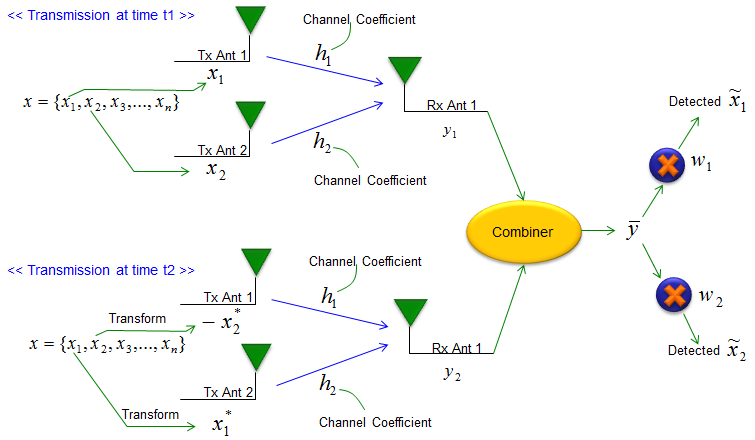
This is my interpretation of the illustration shown above.

i) At higher layer, the exactly same pair of data is transmitted via two Tx antenna twice over two symbol period.

ii) But the transmitted data at the physical antenna has a little different form at each symbol timing. At symbol time t1, the higher layer data is transmitted to each antenna as it is without any modification. but at symbol time t2, the same higher data go through a mathematical changes and also mapping between higher layer data and Tx antenna also changes.

iii) The reciever does not process the data at every symbol. It wait until it recieves two received symbols and combine them in special way and decode each separate transmitted data by using special mathematical process.

Then you may ask 'Why they go through this kind of strange looking and complicated process in stead of simpling transmitting the same data twice or same duplicated data through each antenna ?'

If the radio channel (signal path) is ideal and there is no noise, fading, interference, just transmitting the duplicated data would be OK. Actually if the channel is ideal as it is, you don't even need to transmit the duplicated data since you can guarantee that the transmitted data will be received without any problem and reciever will always successfully decode the transmitted data.

Alamouti invented this method and it is one of the most widely used technique even now (especially in Tx Diversity situation) because it can greatly increase the reliability of recovering the received data in any kind of channel condition.

Then you may ask another question "How can you show (prove) this kind of method can increase the success rate of received data recovery ?".

Now you have to go through all the detailed mathematical process to understand this. If you don't like the math like me :), or does not need that much of the details, you can skip this part and just think 'we use this kind of techniques because it is better in many ways'.

Now let's begin with the math part.

The code matrix and what it costs

The math starts with the shape of what is transmitted. Two symbols go out over two symbol periods from two antennas, and the arrangement of those four slots is the code. Everything later in the derivation follows from that one arrangement.

The drawing below takes the symbol stream x and builds the code matrix from its first two entries.

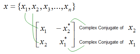
The top row holds what Tx antenna 1 sends, which is x₁ first and then the negated complex conjugate of x₂.
The bottom row holds what Tx antenna 2 sends, which is x₂ first and then the complex conjugate of x₁.
Only x₁ and x₂ appear anywhere in the matrix. The second column carries no new data, which is why the second transmission adds reliability rather than throughput.

The same matrix is worth reading along both of its axes, and the drawing below labels them.

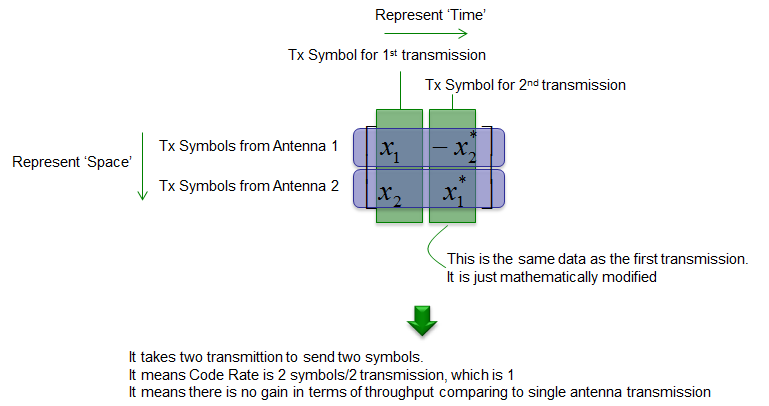
Moving down a column is moving across space, from Tx antenna 1 to Tx antenna 2.
Moving across a row is moving through time, from the first transmission to the second.
The note at the lower right states the cost directly. Two transmissions carry two symbols, so the code rate is 1 and the throughput matches single antenna transmission.

That last line is the honest summary of what Alamouti buys. It buys reliability, and it buys no throughput at all. Sending two different symbols from the two antennas would double the rate instead, and the receiver would then have to separate them with no help from the code.

Writing the two received symbols

The receiver has one antenna, so it hears one value per symbol period. Two periods therefore give it two numbers, y₁ and y₂. The derivation below turns that pair into a form that can be solved for x₁ and x₂.

The compact statement comes first. The received pair equals the channel row times the code matrix, plus noise.

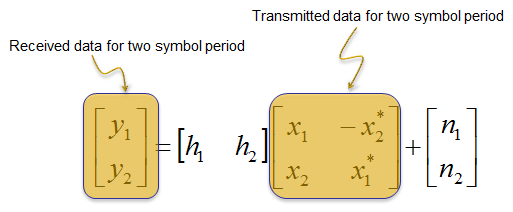
One caution on the shapes in that drawing. The row [h₁ h₂] multiplied by the two by two code matrix produces a row, while the left side is drawn as a column. The drawings below write the same thing one symbol period at a time, and those are the ones to follow.

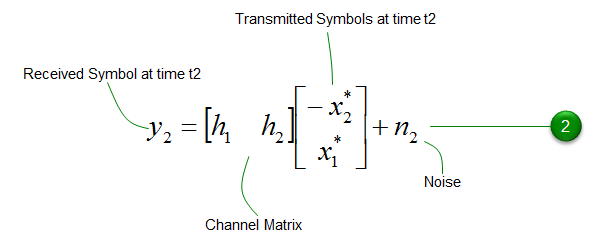
Splitting that by symbol period gives two equations, marked 1 and 2 in the drawings below.

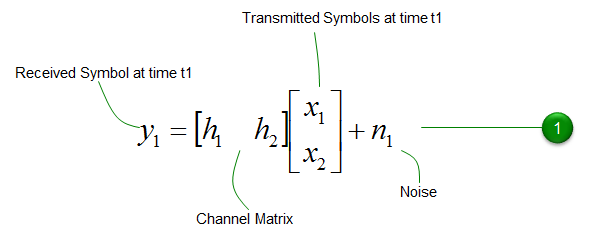
Equation 1 covers the first period, giving y₁ as [h₁ h₂] times the column [x₁; x₂], plus n₁.
Equation 2 covers the second period, giving y₂ as [h₁ h₂] times the column [-x₂^*; x₁^*], plus n₂.
Both use the same channel row, because h₁ and h₂ are assumed constant across the two periods.

The two equations cannot be stacked as they stand, because the unknown vector differs between them. The drawing below states the target shape, with question marks where the answer has to go.

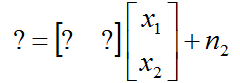
Equation 2 has to be rewritten so that its unknown vector becomes [x₁; x₂], the same one equation 1 already uses.

The rewrite takes three steps, and the drawing below labels them a to d.

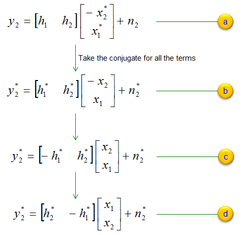
Step a is equation 2 as it stood.
Step b conjugates every term, which turns the unknowns from -x₂^* and x₁^* into -x₂ and x₁.
Step c swaps the order of the two unknowns and moves the minus sign onto h₁^*.
Step d puts them in the wanted order, giving y₂^* = [h₂^* -h₁^*] times [x₁; x₂], plus n₂^*.

Note what ends up stacked. It is not y₂ but its conjugate y₂^*, so the receiver has to conjugate the second sample before combining.

Equation 1 and step d share the same unknown vector, so the two of them stack into one matrix equation.

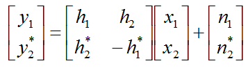
That matrix is the whole point of the code. The receiver now holds two equations in two unknowns, taken from a single receive antenna over two symbol periods.

Why the two columns are orthogonal

Two equations in two unknowns can always be solved by inverting the matrix. Alamouti never inverts anything, and the reason is a property of that matrix itself.

The drawing below names the two columns c₁ and c₂ and states the property.

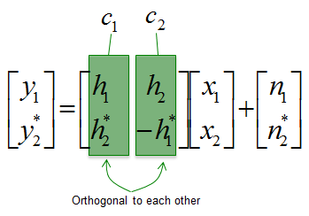
c₁ is the column [h₁; h₂^*] and c₂ is the column [h₂; -h₁^*]. The note underneath claims that the two are orthogonal to each other, whatever values h₁ and h₂ happen to take.

The proof takes one line, and the drawing below works it through.

Taking the Hermitian of c₁ gives the row [h₁^* h₂], and multiplying that by c₂ gives h₁^* h₂ plus h₂ times minus h₁^*. The two terms are the same product with opposite signs, so the result is zero for every channel.

That is what the O in OSTBC stands for. The orthogonality holds by construction rather than by chance, so the receiver never has to ask whether the matrix is well conditioned. Compare that with the Zero Forcing page, where a poorly conditioned channel matrix is exactly what amplifies the noise.

The property also settles how many antennas the scheme can use. A two by two code matrix with orthogonal columns exists for two transmit antennas at a rate of 1, and no such code exists for more than two antennas at that rate. Larger OSTBC designs therefore have to give up rate, which is why the two antenna case is the one the standards adopted.

Recovering x1 and x2

Orthogonal columns mean that projecting the received vector onto one column removes the other completely. The two weight vectors below are those projections, each normalised so that the combining does not scale the noise up.

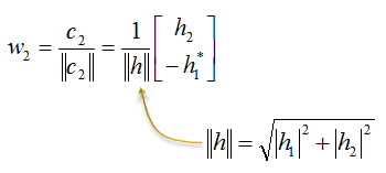
Each weight vector is its own column divided by that column's length, and the two lengths are equal. The drawings below give w₁ and w₂.

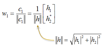
The first weight vector w₁ is c₁ divided by its norm, which is 1 over ||h|| times the column [h₁; h₂^*].
The second weight vector w₂ is c₂ divided by its norm, which is 1 over ||h|| times the column [h₂; -h₁^*].
||h|| is the square root of |h₁|² + |h₂|². Both columns share it, because both hold the same two coefficients.

Applying w₁ to the stacked received vector recovers the first symbol. The drawing below carries the steps.

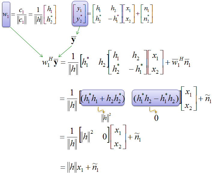
The first bracket collapses to ||h||² and the second collapses to zero. The orthogonality proved above is what forces that second bracket to zero. What remains is ||h|| x₁ plus a noise term, so x₁ arrives scaled by ||h|| and free of x₂ entirely.

The second symbol follows by the same route, with w₂ in place of w₁.

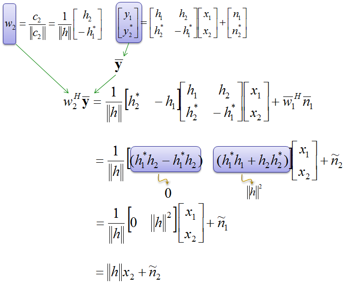
This time the first bracket is the one that collapses to zero and the second gives ||h||², so the result is ||h|| x₂ plus noise.

That last drawing carries two label slips worth knowing. The noise term on its third line is written with w₁ and n₁ where it should carry w₂ and n₂, and the line above the result still reads n₁ tilde rather than n₂ tilde. The final line is correct.

The gain sits in the ||h|| factor. Both symbols come out multiplied by the square root of |h₁|² + |h₂|². A deep fade on one path therefore does not by itself lose the symbol, provided the other path is not faded as well. That is the diversity, and it cost no channel knowledge at the transmitter and no feedback.