STBC is a kind of coding scheme for TX diversity or MIMO and I hope you can figure out the meaning of STBC directly from following illustration. Just connect the words in red -:). In short, STBC is a multi Antenna technique in which a multiple symbols are transmitted as a block (2 D array) of multiple Antenna (representing Space) and Symbol Time. There can be different ways on how to arrange the symbols within the block to be transmitted. One of the most common arrangement is as in Figure 1. This is called Alamouti code.

• How the block is arranged
• The other way the matrix is written
• Why this particular block ?
• What breaks it, and why LTE uses SFBC

How the block is arranged

In the following illustration(example), x represents 'bit' and s represent a symbol. You would notice one bit is mapped to one symbol, so this example is for BPSK.

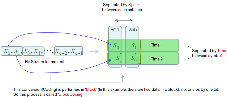
Figure 1. The name read off the picture. One block of two symbols is spread over two antennas, which is the space part, and over two symbol times, which is the time part. The three words in red spell out Space, Time and Block.

• Read the grid as antennas across and symbol times down : at Time 1 Ant 1 sends s₀ and Ant 2 sends s₁. At Time 2 Ant 1 sends -s₁^* and Ant 2 sends s₀^*.
• The second row is not a repeat of the first : it carries the same two symbols in the opposite order, conjugated, with one sign changed. Those three changes are what the receiver exploits.
• Two symbols occupy two symbol times : the block sends one symbol per time slot on average, so the coding costs no rate at all.
• Block means two symbols at a time : the note along the bottom says the coding is performed in a block rather than one bit by one bit. A block holds two here.
• The bit stream along the left reads x₀, x₁ then x₃, x₄ : the second pair should be x₂, x₃ for the blocks to tile the stream without a gap. The same slip appears in the matching figure on the SFBC page.

Two properties of that arrangement matter, and the picture shows neither. The first is that the two rows are orthogonal when read as vectors, which is what lets a receiver separate s₀ from s₁ without inverting anything. The second is that each symbol leaves from both antennas, once directly and once conjugated, so each symbol travels two independent paths.

Those two properties together are the whole of the scheme. Rate is unchanged, two paths carry every symbol, and the receiver needs one multiplication rather than a matrix inverse. The section below the notation works out why the arrangement delivers them.

The other way the matrix is written

In some material, you may see this matrix represented as shown below. Basically it doesn't matter whether you present as in Figure 1 or as in Figure 2, but you have to be careful about writing mathematical process in channel modeling.

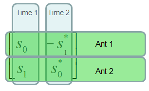
Figure 2. The same code with the axes exchanged. Time runs across the columns here and the antennas run down the rows, which is the reverse of Figure 1. The two pictures hold the same four entries.

• Row Ant 1 reads s₀ then -s₁^* : that is the left column of Figure 1 laid on its side. Row Ant 2 reads s₁ then s₀^*, which is the right column.
• One matrix is the transpose of the other : nothing has been renamed, negated or conjugated between the two figures, so both describe the same transmission.
• This is the form most papers print : a row per antenna reads naturally as what each antenna transmits over time, which is why the literature usually chooses it.

The care the paragraph above asks for has a specific form, and it is worth stating so that it can be checked. The two pictures are transposes of each other, so the matrix sits on a different side of the channel in each case.

Take h₀ and h₁ as the channel from antenna 1 and antenna 2. With the Figure 1 layout, rows are time and the received pair is the matrix times the channel written as a column. With the Figure 2 layout, rows are antennas and the received pair is the channel written as a row times the matrix. Both give y₁ = h₀s₀ + h₁s₁ and y₂ = -h₀s₁^* + h₁s₀^*.

The trap is mixing them. A matrix copied from one source and a formula copied from another silently transposes the code, which exchanges the two antennas and moves the minus sign to the wrong branch. The result is still a valid Alamouti code and it no longer matches the picture it was taken from, so every later expression disagrees with the figure by a transpose.

• Fix one layout before deriving anything : rows as time or rows as antennas, either is fine, and mixing the two is what goes wrong.
• Check the convention against the picture : read off which antenna carries the negated conjugate, and confirm the formula puts it there.
• A transposed code still works : that is what makes the mistake hard to notice, because nothing fails until the algebra is compared with the drawing.

Why this particular block ?

Now you may ask "Why they use this kind of specific block (array) ?".. "how do they guarantee that this kind of block transmittion gurantees the improved performance ?" This is the part where you need to go through a thick book and a lot of mathematic formulas to find the answer. I would not go through these topics for now.

Just for now, you can only take it as a proven technology in theory and widely used in the industry.

If you are really interested in the details (theory), you may read Alamouti Code/OSTBC page as an example.

The short answer fits on this page, and it needs no thick book. The arrangement is chosen so that the two rows of the block are orthogonal, and orthogonality is what turns a joint search over symbol pairs into two separate single symbol decisions. Figure 3 carries out the whole receiver in three steps.

Start with what arrives. At Time 1 both antennas transmit, so the receiver collects y₁ = h₀s₀ + h₁s₁ plus noise. At Time 2 the block sends the conjugated pair, so it collects y₂ = -h₀s₁^* + h₁s₀^* plus noise. One equation is linear in the symbols and the other is linear in their conjugates, which is why the pair cannot be solved as it stands.

Conjugating the second equation fixes that, because y₂^* becomes h₁^*s₀ - h₀^*s₁ plus conjugated noise. Both lines are then linear in s₀ and s₁. Two equations in two unknowns follow, and the particular coefficients make them trivial to separate.

Figure 3. The whole receiver, in three steps and no matrix inverse. Conjugating the second sample makes both lines linear in the same two symbols, after which one weighted sum recovers each symbol with the other cancelled exactly.

• Each weighted sum keeps one symbol and cancels the other : the cancellation is exact rather than approximate, and it holds for every channel rather than for favourable ones.
• The surviving gain is the same in both : g is the sum of the two squared channel magnitudes, so each symbol arrives having travelled two independent paths added in power.
• No matrix is inverted anywhere : the receiver multiplies and adds, which is the saving the orthogonal arrangement buys over an arbitrary one.
• Conjugating the second sample is the step that makes it work : without it the two equations describe different unknowns and no combination separates them.

That answers the second question in the paragraph above as well. Each symbol reaches the receiver multiplied by the sum of two squared channel magnitudes rather than one. The diversity order is therefore two, and a deep fade now requires both paths to fail at once. The SFBC page puts numbers on what that is worth, because the same combining appears there.

The arrangement does not buy extra average power. Two antennas share the power one antenna would have used, so the mean received power is unchanged and the gain sits entirely in how rarely the channel collapses. That is the correct reading of proven technology in the paragraph above.

What breaks it, and why LTE uses SFBC

One assumption ran through Figure 3 without being stated. The same h₀ and h₁ appear in the Time 1 line and the Time 2 line, so the channel was taken to be identical in both slots. Everything the block delivers rests on that, and a moving terminal does not supply it for free.

The first result runs against expectation. A phase rotation applied equally to both antennas cancels completely, because the off-diagonal term is a difference of two products that both pick up the same unit factor. Over 5000 random channels with a random common rotation the largest off-diagonal term came to 1e-15, which is arithmetic noise. A shared frequency offset or a drifting oscillator therefore does not disturb the cancellation at all.

What does disturb it is the two paths changing differently between the slots. Antenna 1 and antenna 2 see different scatterers, so their channels decorrelate at a rate set by the Doppler spread. Once they do, the two products stop matching and the other symbol leaks in. Two symbol times span at least 133 microseconds, since one useful OFDM symbol is one divided by 15 kHz, and the cyclic prefix adds to that.

The table puts numbers on it, using the standard Jakes correlation over that interval at a 2 GHz carrier. The leakage is given relative to the wanted term, so a larger number is better.

• A common phase rotation costs nothing : both products pick up the same factor and the difference stays zero, so oscillator drift and a shared frequency offset do no harm.
• Decorrelation is what actually costs : the two antennas have to stay in the same relationship to each other, which is a stronger demand than either staying still.
• Walking pace is safe and a train is not : the margin falls from 54 dB at 3 km/h to 15 dB at 300 km/h. Self interference 15 dB down is inside the range that limits a link.
• The interval is fixed by the numerology : two symbol times cannot be shortened without changing the subcarrier spacing, so the exposure is not something a designer can remove by tuning.

That exposure is the reason this page sits slightly apart from LTE practice. LTE transmit diversity does not place the block in time. It places exactly this block on two adjacent subcarriers within one OFDM symbol, which is SFBC rather than STBC, and the arithmetic of the combining is unchanged.

Moving the pair into frequency exchanges one condition for another. The time version needs the channel steady across 133 microseconds and is exposed to Doppler. The frequency version needs it flat across 15 kHz and is exposed to delay spread instead. The frequency against time section compares the two directly, and the frequency placement has the further advantage of completing inside one OFDM symbol, so no scheduler can split it.

The material above transfers directly. The block in Figure 1, the notation in Figure 2 and the receiver in Figure 3 are the same in both schemes, and only the axis the pair is laid along changes. Alamouti is the name of the arrangement rather than of the axis, which is why the Alamouti Code/OSTBC page the author links above covers both.

• LTE uses the frequency version of this block : the same two by two arrangement, laid across two subcarriers rather than two symbol times.
• The receiver arithmetic does not change : Figure 3 applies to SFBC with the two subcarrier samples in place of the two time samples.
• Each version has its own exposure : Doppler for the time placement and delay spread for the frequency one, and LTE is designed for terminals that move.