Zero Forcing Model

In this page I will explain about Zero-Forcing Technology. It might be a kind of simplest model both in conceptually and mathematically, but it has a serious drawback called 'Noise Amplification'. But there are many cases where these technique is used for simplicity and in terms of learning the channel modeling theory it can be a good starting point to study. (You may already have questions like 'why it is called Zero-Forcing ? What is the practical meaning of Zero-Forcing ? Why this technology can cause Noise Amplification ? Just keep all these questions in your mind. Some of the questions will be answered automatically on the way through the mathematical process).

I will start out with the ideal/the simplest case and expend it to more complicated but more realistic model as follows.

What is it ? and Why Zero Forcing ?

The Zero Forcing (ZF) channel model is a linear equalization technique used in wireless communication systems to mitigate the effects of intersymbol interference (ISI) and co-channel interference. These issues arise when multiple signals transmitted simultaneously over the same channel overlap and interfere with each other. The ZF channel model aims to eliminate or minimize such interference by inverting the channel matrix.

In the context of multiple-input multiple-output (MIMO) systems, where multiple antennas are used for both transmission and reception, the ZF equalizer uses the inverse of the channel matrix to pre-process the received signals. This processing effectively "forces" the interference components to zero, hence the name "Zero Forcing."

The Zero Forcing channel model is still widely used due to its simplicity and effectiveness in reducing interference in certain scenarios. It is often employed as a benchmark to evaluate and compare the performance of other equalization techniques.

The Zero Forcing (ZF) equalizer attempts to minimize the interference by inverting the channel matrix. Inverting the channel matrix H allows us to "undo" the effect of the channel on the transmitted signal X, so that the received signal Y can be used to reconstruct the original transmitted signal with minimal interference.

Let's think of simple system equation as below :

Y = H * X + N ,

where Y is the received signal, H is the channel matrix, X is the transmitted signal, and N is the noise vector.

Multiplying the H^-1 on both side, we get

H^-1 * Y = H^-1 * (H * X + N)

Expanding the equation we get

H^-1 * Y = H^-1 * H * X + H^-1*N

Rearranging Equation

H^-1 * H * X = H^-1 * Y - H^-1*N

Replacing H^-1 * H with I (Identity Matrix)

I * X = H^-1 * Y - H^-1*N

Simplifying

X = H^-1*Y - H^-1*N

Drawbacks of Zero Forcing ?

Inverting the channel matrix solves the interference problem exactly. It does not solve the noise problem, and it makes the noise problem worse. The three drawbacks below all follow from that one inversion, so they are worth reading together rather than as a list of unrelated faults.

The ZF channel model has certain drawbacks:

Noise amplification: When the channel matrix has a small singular value or is ill-conditioned, the inversion process can lead to significant noise amplification, which degrades the performance of the system. ==> If the determinant of H matrix is small, the term H^-1*N gets large. this is the noise amplification.
Computational complexity: Calculating the inverse of a large matrix can be computationally intensive, especially for real-time applications.
Suboptimal performance: The ZF equalizer does not take into account the noise statistics, which can result in suboptimal performance compared to other equalization techniques like the Minimum Mean Squared Error (MMSE) equalizer.

Noise amplification is the one that decides whether ZF is usable at all. The other two are engineering costs, and both of them can be paid. Matrix inversion is expensive, but the cost is known in advance and the hardware can be sized for it. Ignoring the noise statistics costs a fixed margin against MMSE, and that margin can be measured once. Noise amplification behaves differently, because its size depends on the channel and the channel keeps changing.

The quantity that governs it is the condition number of H, which is the ratio of the largest singular value to the smallest. A well conditioned channel amplifies the noise a little. An ill conditioned channel amplifies it without any bound, and the receiver output becomes noise rather than data. Two antennas that see almost the same propagation path produce exactly that, and antenna spacing is the usual reason.

Same number of Tx and Rx Antenna without Noise.

There are many real case where the same number of Tx antenna and the same number of Rx Antenna are used but there would rarely the case where there is no noise. But I will start out this case to mathematical process simpler and make it easier to understand.

Let's start with simplest and almost an ideal case where number of Tx antenna is same as number of Rx antenna and there is no noise in the channel. More specifically, let's assume the case with 2 x 2 MIMO case. It means two Tx antenna and two Rx Antenna.

In this case, the channel model can be described as follows (If you are not familiar with how this expression comes out, refer to Channel Model Overview section). The important thing to notice is that in this case the channel matrix H is a square matrix. Also, you would notice that there is no Noise term in the equation since we assume the case where thes is no Noise.

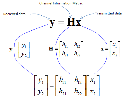
This is the system equation for this channel and it is the end of channel model. Simple enough ?

Now let's suppose that we need to find way to figure out the transmitted data from this channel model. This is the goal of reciever design.

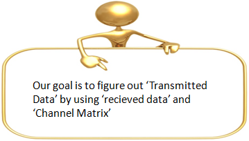
Assuming that we already have all the information on channel marix (H), now the problem is just to solving the following equation in terms of x. i.e, figuring out 'x' in the following equation. (You may ask how can we know of 'H', but let's just assume that it is already given to us. It is another big topic which should be covered as a separate page).

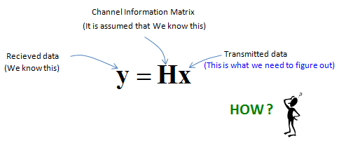
Since the number of Tx and Rx antenna are same, H is a square matrix. Getting 'x' from the above would be simple as you might have learned from an elementry linear algebra course.

The solution process for this case can be summarized as below.

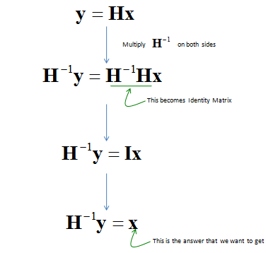
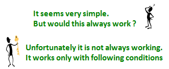
It may look simple, but there are special condition in which a problem can be solved like this method. The conditions is summarized as below.

Same number of Tx and Rx Antenna with Noise.

Now let's think about the case where Noise is added to the case described above. In this case, we cannot solve the equation directly because of the noise term. The noise term can be estimated only by statistical method and this estimation process can be described as follows.

The two derivations below run in sequence. The first one multiplies both sides by H^-1 and isolates the term H^-1*n, which cannot be calculated directly because n is unknown. The second one takes the covariance of that same term and reduces it to a form that depends only on H and on the noise variance.

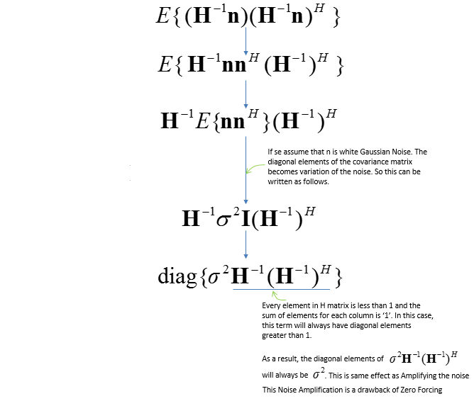
The first derivation reaches H^-1*y = x + H^-1*n. The identity matrix has already absorbed H^-1*H, so only the noise term is left to deal with.
The second derivation assumes that n is white Gaussian noise. Its covariance E{n n^H} then becomes sigma² times the identity matrix, and the whole expression collapses to sigma² * H^-1 * (H^-1)^H.
The diagonal of that matrix is what the receiver sees as noise power. The note at the lower right states that these diagonal elements are always larger than sigma², and that is the noise amplification named in the previous section.

The final equations would become as follows.

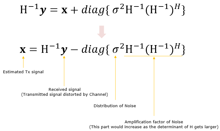
The yellow labels under the final equation name each term. Reading from the left, they give the estimated Tx signal, the received signal, the distribution of the noise, and the amplification factor.

One caution on that last label. The drawing says the amplification factor grows as the determinant of H gets larger, and the relation runs the other way. A small determinant makes H^-1 large, and a large H^-1 is what amplifies the noise. The bullet in the drawbacks section above states it correctly.

Different number of Tx and Rx Antenna without Noise.

Now let's look into a case where we have non square channel matrix. We will look into following cases as an example. As you see, we have two transmitter antenna and four reciever antenna, meaning that the number of transmitter antenna and reciever antenna is not same.

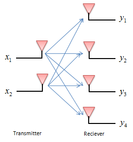
By now you should be able to build a channel matrix for whatever configuration is given to you. If not, try more practice on creating a channel matrix for various transmitter and reciever combination. The channel matrix for this case is as follows.

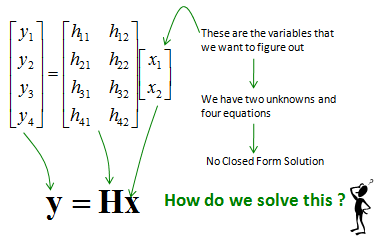
As you see, the channel matrix is not square. We have two variables (unknowns) that we want to figure out, but we have four equations. This is what they called 'over determined' case in linear algebra course. In this case, we cannot have any analytic solution (exact solution) since the inverse of the channel matrix does not exists.

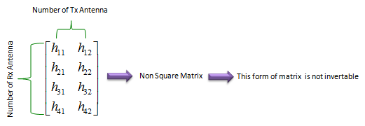
In this case, you cannot get any exact solution (exact answer), but you can have a approximate answers with various techniquest. One of the common techniques we use in this case is "Least Square Error" method and the overall logic is as follows.

Let's first check on what we know and don't know. 'y' is a know value(vector) since it is what was recieved/measured by the reciever antenna. We also assume that H is known as well. 'x' is unknown for now and this is what we need to figure out.

Now let's try a funny thing. Since there is no analytic solution to figure out 'x' in this case. Let's assume that we make a guess and plug in any guessed number in it. Now we have two parts, one is 'y' which is from direct measurement and another part 'Hx' which is calculated from H and the guessed value 'x'. Since 'x' can only be approximate value in this case, if you take the difference between y and Hx, you would always have some non-zero value. We call the valu as an error. If we express this in mathematical form, it becomes as follows.

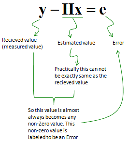
Keep making guess for x and plugging in the guessed x and calculate the error value.. if you keep trying this almost infinate times and get the guessed x value which produced the least number of e (Error), you can call it the best approximate answer to this equation. But if you do this kind of blind guessing work, it would take forever to find answer.

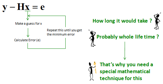
In stead of doing endless wild(blind) guess, let's use a mathematical approach for this. Our goal is to find 'x' that makes 'e' to be the minimum. By squaring both side, we can have a mathmatical form the min (or max) of the value can be analytically found. (If you are not familiar with Least Square Error method, your first question would be 'why we need to get the equation squared ?'. It is very good question and important question.. but I would not explain about it in detail since it would deviate our topic too much. However, I strongly recommend you to try read some materials about 'Least Square' or 'Least Square Error' method).

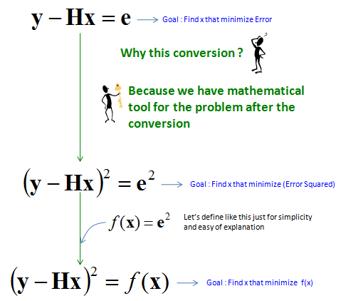
Now our original problem boiled down to find 'x' that gives the minimum value of a quadratic function as illustrated below.

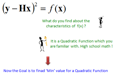
From high school math, you would recall that in any quatratic function.. the first derivative (slope of tangential line) of the function becomes 0 at the min (or max) location.

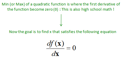
By a long and tedius process (I would not go all the steps not to get you bored out), it would give you final answer as shown below. The important thing is that you can get the best approximate of 'x' just from 'y' and 'H'. There would be anybody who may not familiar with another symber 'H' in the superscript.. it is 'Hermitian' matrix symbol. If you can guarantee that the channel matrix has real values at all it's element, you can use 'Transpose' matrix, but it cannot cover the case where the channel matrix has any complex number element. So it would be safe to use Hermitian matrix which can handle both real matrix and complex matrix.

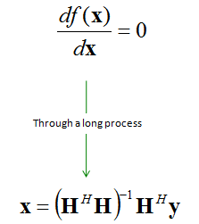
Even though it would looks to be long/confusing/scary/tedious process, this is one of the simplest methods. It is simple, but it cause some issues at some specfic case.. so they developed a little more complicated but more robust method called 'MMSE' on which I will explain later.

Different number of Tx and Rx Antenna with Noise

This is the case that a real receiver actually meets. The channel matrix is not square, and the received vector carries noise. Neither of the two previous sections covers it on its own, but the two of them together give the whole answer.

Start again from y = H * X + N, with H now taller than it is wide. The inverse of H does not exist, so the step used in the square case is not available here. The least square solution from the previous section replaced it, and that expression is still defined when noise is present. The matrix (H^H * H)_inv * H^H is called the pseudo-inverse of H, and it is usually written as H⁺.

Substituting y = H * X + N into that solution shows what the noise does. The result is X_est = X + H⁺ * N, which has the same shape as the square case. The estimate splits into the true transmitted vector plus a noise term, and the noise term is the pseudo-inverse acting on N. Nothing about the non square shape removes the amplification.

The same quantity governs how large that term gets. Take the covariance of H⁺ * N under white Gaussian noise. The result is sigma² * H⁺ * (H⁺)^H, which is the expression from the square case with H⁺ in place of H^-1. Its diagonal elements are the per stream noise powers at the receiver output. A channel matrix with two nearly identical columns gives large entries there, whatever the number of Rx antenna is.

Extra Rx antenna do help, and this is where the non square case differs from the square one. Four Rx antenna carrying two streams give the least square fit four measurements to work from instead of two. The fit averages the noise across all four, so the diagonal entries come out smaller than a 2 x 2 channel of the same conditioning would give. The gain comes from the extra rows, not from the inversion itself.

ZF reaches its limit here. The pseudo-inverse minimizes the squared error between y and H * X, and it ignores the noise variance completely. MMSE puts that variance into the inversion and trades a little interference for much less noise. That is the method mentioned at the end of the previous section.

Takeaways

A non square channel matrix has no inverse, so ZF uses the pseudo-inverse H⁺ = (H^H * H)_inv * H^H instead.
Noise passes through unchanged in form. The estimate is X_est = X + H⁺ * N, exactly as in the square case.
The noise power at the output is the diagonal of sigma² * H⁺ * (H⁺)^H, so poor conditioning still amplifies the noise.
Adding Rx antenna reduces that noise power, because the least square fit gets more measurements for the same number of unknowns.
ZF never uses the noise variance, which is the gap MMSE fills.