Gradient Descent Method

Many engineering problems come down to one question: which input value makes a cost function as small as possible ? For a simple function you can set the derivative to zero and solve the equation. For a neural network with millions of weights, nobody can solve that equation directly. Gradient descent takes a different path. It starts from a guess and walks downhill one step at a time, using only the slope at the current point.

We'll start with the update rule and what each term does. Then we'll see why the method can stop at a wrong point, and follow it step by step on a quadratic function. The last two sections are about the constant alpha, which decides whether the walk is fast, slow or unstable.

How does the update rule work ?

The whole method is one line of math. Let's read that line term by term, because every later section on this page is a consequence of it.

Gradient Descent Method is a technique to find a minimum value of a function by changing the value of variables repeatedly based on the the following rule.

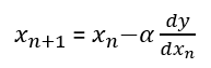
Gradient descent update rule x n plus 1 equals x n minus alpha times dy over dx n

Figure 1. The gradient descent update rule. The next point is the current point minus alpha times the slope at the current point.

If you can make any sense out of this equation just by looking at this equation, you don't have the read this page any more.

If you still want to get a little bit of further explanation, take a look at following.

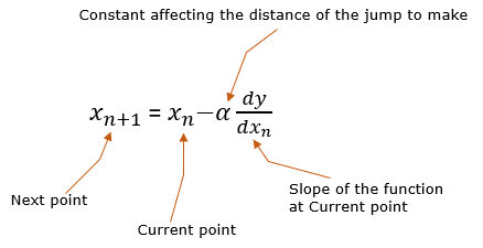
Update rule annotated with next point, current point, constant alpha and slope at the current point

Figure 2. The four parts of the update rule. Alpha and the slope together set the distance of the jump.

Now I hope you got a little bit of more concrete idea, but I think you still want to get some more details. I hope following would help you a little bit further.

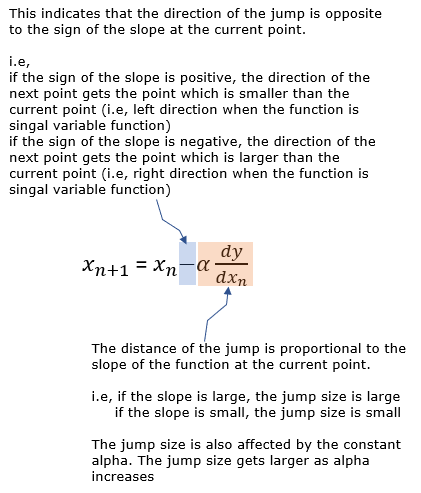
Update rule annotated with the direction of the jump from the minus sign and the size of the jump from alpha times the slope

Figure 3. Direction and size of the jump. The minus sign sends the point against the slope, and the slope and alpha set how far it goes.

The minus sign always points downhill : a positive slope moves x to the left, and a negative slope moves x to the right. Both moves go toward lower values of y.
A steep slope gives a long jump : far from the minimum the slope is large, so the point moves fast. Near the minimum the slope is small, so the steps shrink by themselves.
Alpha scales every jump : alpha is the one value you choose. The section Effect of the Alpha shows what happens when it is too small or too large.
More variables, same rule : for a function of several variables, dy/dx becomes the gradient, the vector of partial derivatives, and each variable is updated with its own partial derivative.

Why can the method stop at a wrong point ?

The rule moves the point only while the slope is not zero. That is exactly what we want at the minimum. But the slope is also zero at other points, and the rule cannot tell those points apart from the minimum.

NOTE : At this point, we need to notice a very important point. As mentioned above, the step size (distance of jump) is determined by the constant alpha and the slope of the function (dy/dx). It implies the following two points

i) if alpha is set to 0, the step size gets 0 meaning the point(x) does not move

ii) if dy/dx gets 0, the step size gets 0 meaning the point(x) does not move

We don't worry about the point i) because the alpha is completely under our control and we wouldn't set it to zero. The important thing is the point ii). This property acts as a advantage or disadvantage depending on the situation. The minimum position of any differentiable funtion always have the slope 0 at the point. This is good because this make the point does not move away once it reaches the minimum point. But not every points with the slope 0 is minimum value of the function. For example, let's suppose we have a function as shown below (black curve). In this function graph, you can see 5 position where the slope(dy/dx, gradient) gets 0. If you reach any of these points, you get stuck there (i.e, does not move any more) because the jump size gets 0 due to dy/dx. If you are at (A) and stuck there, it is lucky because it is the real(global) minimum of the function, but if you are at any other points, you get stuck at a wrong point.

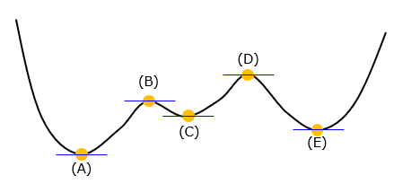
Curve with five zero slope points A to E, one global minimum, two local minima and two local maxima

Figure 4. Five points with zero slope. Only (A) is the global minimum, but the update rule stops at any of them.

(A) is the global minimum : it is the lowest point of the whole curve, and it is the point the method is meant to find.
(C) and (E) are local minima : each one is the lowest point in its own valley. A walk that starts in one of these valleys ends there, because every step goes downhill.
(B) and (D) are local maxima : the slope is zero, but any small move away from them goes downhill. So the walk stops there only if it lands exactly on them, which rarely happens in practice.
The starting point decides the valley : with a small alpha, the walk stays in the valley where it starts. The Effect of the Alpha section shows that a large alpha can jump over a hill into another valley.

How does the method walk down a quadratic function ?

A quadratic function has only one valley, so nothing can go wrong in the way Figure 4 shows. That makes it the right function for watching the rule work step by step. The plots below use y = x², whose slope is dy/dx = 2x.

Now let's confirm this explain with a concrete example. Let's assum that you have a quadratic function and you set the initial point as shown below. From this initial point, you have to determine the next point as commented below (try to associate this comments with the mathematical expression shown above).

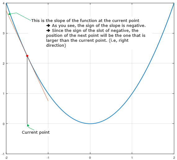
Quadratic curve with the current point at x equal to minus 1.5 and the tangent line showing a negative slope

Figure 5. The first point at x = -1.5. The tangent has a negative slope, so the next point lies to the right.

By this logic, you can get the next point as shown below.

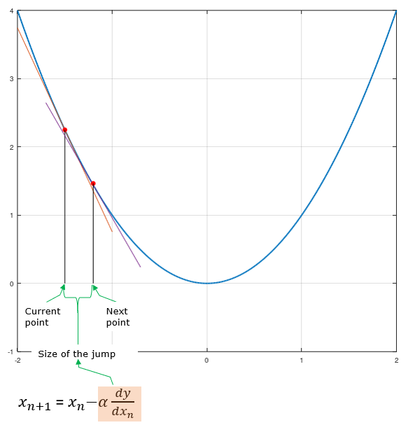
Quadratic curve with the current point, the next point and the size of the jump between them

Figure 6. The first jump. The point moves from x = -1.5 to about x = -1.2, and the jump size is alpha times the slope.

Then from the second point you found, apply the same logic repeatedly until you reach the minimum point of the function. Following plot shows the example of several steps for this function and shows how the slope of the function at each point affects the size of the jump. (NOTE : Click on the graph or here to see the slide show or animation version of this process).

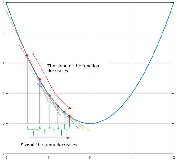
Figure 7. Six points of the walk. The slope drops at every step, so the jumps get shorter as the point nears the minimum.

Let's check the plot with numbers. The points in Figure 7 sit at x = -1.5, -1.2, -0.96, -0.768, -0.614 and -0.492, with y = 2.25, 1.44, 0.92, 0.59, 0.38 and 0.24. These values fit alpha = 0.1. With that alpha, the rule becomes x_n+1 = x_n - 0.1 x 2x_n = 0.8 x_n. So every step keeps 80% of the remaining distance to the minimum at x = 0. The jumps are 0.3, 0.24, 0.192 and so on, and each one is 80% of the one before.

NOTE : Now the last step for you to get the complete understanding is to go through many examples. The best way would be for you to create those examples on your own, but as a second best one I have made those examples for you in slideshow format in my visual note www.slide4math.com . Go to [Engineering]->[2]->[Gradient Descent].

The step shrinks without any change to alpha : alpha stays at 0.1 the whole time. The jumps get shorter only because the slope 2x gets smaller.
The approach is geometric : the distance to the minimum is multiplied by 0.8 at each step, so the point gets close quickly but never lands exactly on x = 0.
A stopping rule is needed : in practice the loop stops when the step, or the slope, falls below a small threshold.

Effect of the Alpha

What I want to talk in this section is about the effect of Alpha in the following equation on the speed of finding the minimum value of a function.

Gradient descent update rule x n plus 1 equals x n minus alpha times dy over dx n

Figure 8. The same update rule as Figure 1. This section changes only alpha.

Based on the equation above, the speed of the finding the minimum value is affected by the slope (dy/dx) and the constant alpha. The effect of the slope is briefly described at this NOTE. The effect of Alpha will be explained in this section. In fact, the role of Alpha is much more important in gradient descent algorithm and finding the proper Alpha value in most practical application is not easy.

NOTE : One of the most important application of the Gradient Descent method would be Neural Network. The constant alpha is called Learning Rate and it is very, very important parameter you have to specify properly in Neural Network. What you will learn in this section would be helpful to understand how network parameters (e.g, weights and bias) in Neural Network is calculated and updated.

Let's take a look at a simple example as shown below (You can see this example in slideshow in this page in my visual note www.slide4math.com). The goal here is to find the minimum value marked as a blue star and the red dots shows the process of each steps to reach the goal (the black line is connecting the dots of the gradient descent process). The plot (A) and (B) shows the process of gradient descent process with two different Alpha value. (B) uses larger Alpha value than (A). You see that the large Alpha let you find the min value faster.

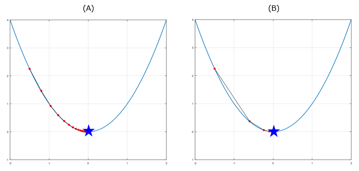
Gradient descent on a quadratic with a small alpha in plot A and a larger alpha in plot B

Figure 9. Plots (A) and (B). A larger alpha reaches the minimum in fewer steps while the steps stay on one side of it.

From the above examples, it seems that large Alpha value result in faster min finding. Would this be always true ? Let's increase the Alpha value a little bit further (C) is using the alpha value a little bit larger than the case (B). You see this reaches the min value faster than (A) at least but the path to find the value looks a little strange. Now let's push up the Alpha value further as shown in (D). (D) uses the Alpha value much greater than (C). As you notice here, the path to reach the goal swings back and forth and takes much longer to reach the goal. This example shows simply increasing the Alpha value does not necessarily helps to find the min value quickly.

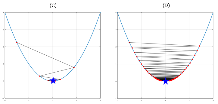
Gradient descent on a quadratic with a large alpha in plot C and a much larger alpha in plot D, both jumping across the minimum

Figure 10. Plots (C) and (D). Past a certain alpha, every step jumps over the minimum, and a slightly larger alpha makes the swing decay very slowly.

(A) creeps toward the minimum : its points match Figure 7, so alpha is about 0.1 and each step keeps 80% of the distance.
(B) is fast and stays on one side : the second point is at about x = -0.6, which fits alpha = 0.3. Each step keeps only 40% of the distance.
(C) crosses the minimum at every step : the points go from -1.5 to about +0.9 and then to about -0.54, which fits alpha = 0.8. The sign flips, but the distance still shrinks to 60% per step, so (C) is still faster than (A).
(D) almost bounces in place : the second point is at about x = +1.43, which fits alpha of about 0.97. Each step keeps about 95% of the distance, so the walk needs many steps.

Now let's suppose we have a little bit more complicated function as below. (F) uses larger Alpha then (E), but (F) reaches to 'kind of' min location slower than (E). Note that I said 'kind of' min point.. it is not real min value. The real min value is marked as Star shape. In this case, none of (E) and (F) reaches the real min. (Click here or click on the graph to see this plot in slideshow from www.slide4math.com )

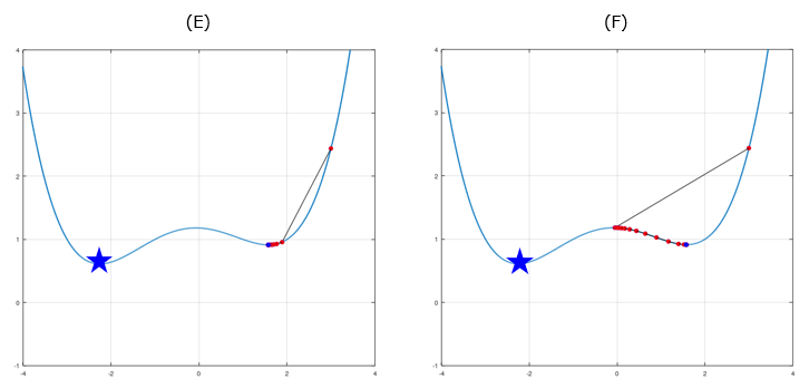
Gradient descent on a function with two valleys where plots E and F both end in the local minimum on the right

Figure 11. Plots (E) and (F). Both walks start at x = 3 and end in the local minimum near x = 1.6, not at the global minimum marked by the star.

Now let's increase the Alpha a little bit. (G) uses an Alpha larger than (F) and (H) use larger value than (G). (G) barely managed to reach the real min (global min) of the function and (H) reaches the global min faster than (G). Then let me ask you the same question again. Do you think simply increasing the Alpha value helps finding the global min faster ? Check on your own in this page.

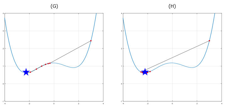
Gradient descent on the same two valley function where plots G and H jump over the hill into the global minimum

Figure 12. Plots (G) and (H). A larger first jump crosses the hill, so the walk ends in the valley of the global minimum.

The first jump decides the valley : at x = 3 the slope is steep, so the first jump is long. In (E) it lands in the right valley. In (F) it lands near the top of the hill, where the slope is small, so the next steps are slow. In (G) and (H) it lands on the left side of the hill.
Reaching the global minimum here is luck, not design : a different starting point or a different alpha could send the same walk into the wrong valley again.

Now let's take a look at a more complicated situation with a case of function of two indepent varaibles. I plot it in a contour plot as shown below. (J) uses the Alpha larger than in (I). In this case, (I) reaches the min value but (J) ends up swinging back and forth between two points (Click here or click on the graph to see this plot in slideshow from www.slide4math.com ).

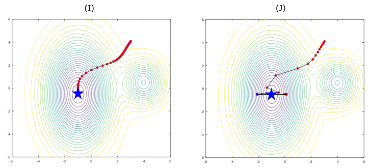
Contour plots of a two variable function where plot I converges to the minimum and plot J swings left and right around it

Figure 13. Plots (I) and (J). With the larger alpha in (J), the walk reaches the valley and then swings left and right across the minimum instead of settling.

Based on several examples show above, do you think there is any general rules on the effect of Alpha on the speed of finding the min value.

Unfortunately No. So finding the best Alpha value would be based on more of trial and error.

Too small is slow : the walk is safe but needs many steps, as in (A).
Too large overshoots : the walk jumps across the minimum, as in (C), (D) and (J), and it can fail to settle at all.
Alpha also changes where the walk ends : on a function with several valleys, (E) to (H) show that alpha changes which minimum the walk finds.

Is there a safe range for Alpha ?

The previous section ends with trial and error, and for a general function that is the honest answer. But a quadratic function gives an exact rule, and that rule also explains the behavior of plots (A) to (D). Near any smooth minimum a function looks like a quadratic, so the rule is a useful guide there too.

Let's take y = c x²/2 with c > 0, so that dy/dx = c x and the second derivative is c. The update rule becomes x_n+1 = x_n - α c x_n = (1 - αc) x_n. So each step multiplies the distance to the minimum by the factor r = 1 - αc. The walk converges only when the size of r is less than 1, which means 0 < α < 2/c. For y = x² in Figures 9 and 10, c = 2 and the safe range is 0 < α < 1.

Alpha for y = x²	Factor r = 1 - 2α	Behavior
0 < α < 0.5	between 0 and 1	Moves toward the minimum from one side, as in (A) with α = 0.1 and (B) with α = 0.3.
α = 0.5	0	Lands exactly on the minimum in one step.
0.5 < α < 1	between -1 and 0	Jumps across the minimum at every step but still converges, as in (C) with α = 0.8 and (D) with α close to 1.
α = 1	-1	Swings between x₀ and -x₀ forever.
α > 1	below -1	Diverges. Each jump lands farther from the minimum than the one before.

The fastest choice is α = 1/c, which lands on the minimum in one step. But you rarely know c in advance, and a real function has a different curvature at each point. For a function of several variables, the curvature is different in each direction. The largest curvature sets the upper limit for alpha, while the smallest curvature sets how slow the walk is along the flattest direction. The swing in plot (J) fits this explanation: the walk settles along one direction of the valley and keeps swinging along the other direction.

The limit is two over the curvature : for a quadratic with second derivative c, gradient descent converges only for 0 < α < 2/c.
Crossing the minimum is not failure : for 1/c < α < 2/c the walk jumps across the minimum at every step and still converges, as plot (C) shows.
The trial and error has a starting point : if you can estimate the largest curvature, start alpha well below 2 divided by that value, then increase it while the cost keeps falling.