Roughly there are two ways to utilize the nerual network. One is to develop the network on your own and the other one is to use various pretrained network. Matlab Machine Learning Toolbox(ML Toolbox) supports the interface functions that let you get access to various pretrained neural net. As of now (Dec 2019), I see around 16 different pretrained neural network that you can utilize using Matlab ML toolbox. See this page for the list of all the pretrained network you can use from Matlab ML toolbox.
This tutorial is to show you a simple example on how you can get access to those pretrained nework and utilize it to classifying your own data. The pretrained network that I am going to use in this tutorial is called Alexnet.
Since the network structure (especially the input layer structure) of those pretrained network differ from each other, you would not be able to copy this example blindly to use other pretrained network, but this example would give you a concrete understandings on overall flow of utilizing a pretrained network.
- Step 1 : Getting Access to the pretrained Network
- Step 2 : Finding the details of the network
- Step 3 : Preprocessing an image to fit to the Input layer requirement of the network.
- Step 4 : Classify my image with the Alexnet
Step 1 : Getting Access to the pretrained Network
First Step is to connect to the Alexnet and store the network to a variable. It is as simple as follows.
alxNet = alexnet
You can print out overall structure of the network simply by printing out the variable.
alxNet =
SeriesNetwork with properties:
Layers: [251 nnet.cnn.layer.Layer]
InputNames: {'data'}
OutputNames: {'output'}
You see that this network is a CNN type of network which is made up of 25 layers.
Step 2 : Finding the details of the network
Then you want to know of the details of each of the layers in the network. That can also be done by printing the layer property of the network variable as below.
alxLayers = alxNet.Layers
alxLayers =
25x1 Layer array with layers:
1 'data' Image Input 227x227x3 images with 'zerocenter' normalization
2 'conv1' Convolution 96 11x11x3 convolutions with stride [4 4] and padding [0 0 0 0]
3 'relu1' ReLU ReLU
4 'norm1' Cross Channel Normalization cross channel normalization with 5 channels per element
5 'pool1' Max Pool 3x3 max pooling with stride [2 2] and padding [0 0 0 0]
6 'conv2' Grouped Convolution 2 groups of 128 5x5x48 convolutions with stride [1 1]
and padding [2 2 2 2]
7 'relu2' ReLU ReLU
8 'norm2' Cross Channel Normalization cross channel normalization with 5 channels per element
9 'pool2' Max Pooling 3x3 max pooling with stride [2 2] and padding [0 0 0 0]
10 'conv3' Convolution 384 3x3x256 convolutions with stride [1 1]
and padding [1 1 1 1]
11 'relu3' ReLU ReLU
12 'conv4' Grouped Convolution 2 groups of 192 3x3x192 convolutions with stride [1 1]
and padding [1 1 1 1]
13 'relu4' ReLU ReLU
14 'conv5' Grouped Convolution 2 groups of 128 3x3x192 convolutions with stride [1 1]
and padding [1 1 1 1]
15 'relu5' ReLU ReLU
16 'pool5' Max Pooling 3x3 max pooling with stride [2 2] and padding [0 0 0 0]
17 'fc6' Fully Connected 4096 fully connected layer
18 'relu6' ReLU ReLU
19 'drop6' Dropout 50% dropout
20 'fc7' Fully Connected 4096 fully connected layer
21 'relu7' ReLU ReLU
22 'drop7' Dropout 50% dropout
23 'fc8' Fully Connec 1000 fully connected layer
24 'prob' Softmax softmax
25 'output' Classification Out crossentropyex with 'tench' and 999 other classes
When it comes to utilizing a pretrained network, the most important thing is to understand all the details of the input layer (layer 1) of the network because you have to preprocess your data according to the requirement of the input layer.
You can print out the details of the input layer (layer 1) by printing out the first element of the variable that stores all the layer information in previous step.
alxInput = alxLayers(1)
alxInput =
ImageInputLayer with properties:
Name: 'data'
InputSize: [227 227 3]
Hyperparameters
DataAugmentation: 'none'
Normalization: 'zerocenter'
NormalizationDimension: 'auto'
Mean: [2272273 single]
In the print out, you see InputSize: [227 227 3]. This mean that this network (a CNN) requires an image with the size of (227 x 227) and with 3 color layer (i.e, RGB color). If you want to save only this inputSize, you can do it as shown below.
alxInputSize = alxInput.InputSize
alxInputSize =
227 227 3
In the same way, you can get the details of the output layer of the network by printing out the last element of the layer array as shown below.
alxOutput = alxLayers(end)
alxOutput =
ClassificationOutputLayer with properties:
Name: 'output'
Classes: [10001 categorical]
OutputSize: 1000
Hyperparameters
LossFunction: 'crossentropyex'
Especially the most important information about the output layer would be the list of the all the category labels of the network. You can figure out all the list of the output label by printing out Class property of the output layer as shown below.
alxCategory = alxOutput.Classes
alxCategory =
10001 categorical array
tench
goldfish
great white shark
tiger shark
hammerhead
electric ray
stingray
cock
hen
ostrich
....
Step 3 : Preprocessing an image to fit to the Input layer requirement of the network.
Now I want to load my own image file that I want to classify with the pretrained network (Alexnet).
First, load an image and store it to a variable as shown below. In order for you to try with your own data (image file in this case), put the image into a folder on your PC and modify the file path according to the location and file name in your PC.
imgfile = sprintf("%s\\temp\\Apple_02.png",pwd)
img = imread(imgfile);
Now I have the make it sure that this image file is in proper format (size and color layers) that fits to the input layer requirement of the alexnet. I hope you remember that the input dimension of the network is 227 x 227 x 3. The image that I am using for this tutorial is already RGB color, so I don't need to do any preprocessing for color layer matching. So I only need to change image size to fit for Alexnet by using imresize() function as shown below.
img = imresize(img,[227,227]);
Plottting the image for check.
imshow(img)

Step 4 : Classify my image with the Alexnet
Now let's put my image into Alexnet and let it classify it. This can be done by the single line as shown below.
[imgClass,imgScores] = classify(alxNet,img);
And you get the result as shown below. imgClass variable stores the label that Alexnet came out with for the image that I put into the network.
imgClass =
categorical
grocery store
imgScores variable returns the scores for the image file that is for each and every labels (i.e, 1000 labels for Alexnet).
imgScores =
11000 single row vector
Columns 1 through 13
0.0000 0.0000 0.0000 0.0000 0.0000 0.0000 0.0000 0.0000 ...
...
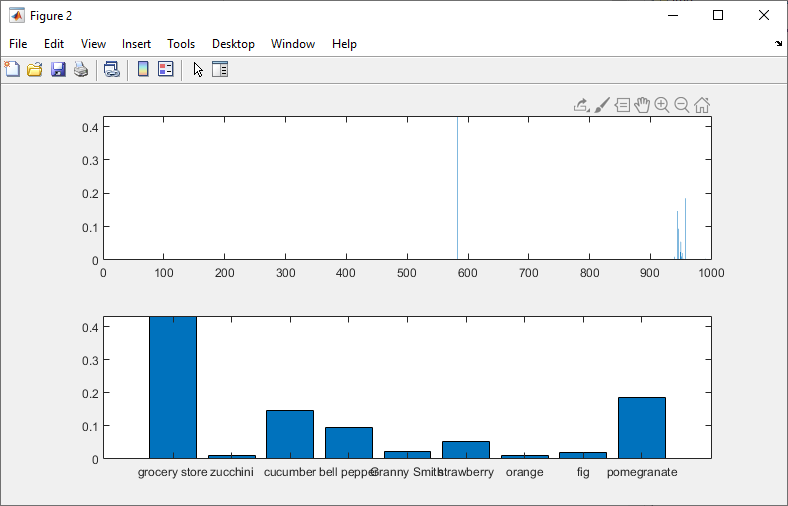
This is not the mandatory step, but let's look into a little bit further into the classification result by plotting the result as below.
In the first plot, I plot the scores of all of the labels of the output layer (1000 labels in Alexnet)
subplot(2,1,1);
bar(imgScores);
In the second plot, I would extract the labels that scores higher than 0.01.
subplot(2,1,2);
imgHighScores = imgScores > 0.01;
bar(imgScores(imgHighScores));
xticklabels(alxCategory(imgHighScores));